
Introduction
Background
Globally, the existence of slums is manifested as a 'normal' but significant part of the contemporary urbanization process and not merely an issue of mismanaged urban planning (Bolay, 2006; Nuissl & Heinrichs, 2013). However, worldwide, the expansion of slums has created issues for policymakers and raised questions for relevant domain-specific research (Marx et al., 2013). In its World City Report of 2022, the United Nations highlighted that the urban population has increased significantly from 25% since 1950, doubling to 50% in 2020 (UN Habitat, 2022). It is expected to grow gradually to 58% in the coming fifty years with the influx of migrants. Urbanization and climate change have altered the morphology of cities and added to urban poverty (Alakshendra et al., 2020; Zelelew & Mamo, 2023). Eventually, the higher demand for housing has increased land prices sharply, reducing the overall supply of affordable housing (O'Hare et al., 1998). As a result, several developing countries, especially in the Global South, are facing rampant growth of slums and informal settlements, indicating poverty and inequality. Hence, through its Habitat III program, the United Nations emphasizes providing access for all to adequate, safe, and affordable housing and basic services, and the upgrading of slums (Smets & van Lindert, 2016).
Along with substandard living conditions, the tenure of rights has been a foundational issue for slum dwellers, Hindman has reported (Hindman et al., 2015). Furthermore, environmental issues in and around slums severely affect the health conditions of the slum dwellers (Vijayalakshmi & Swamy, 2014). Although, the researchers Auyero and Mereine (Auyero, 1999; Mereine Berki et al., 2017) believe that socio-capital and 'interpersonal relations' could assist slum dwellers to battle extreme poverty, these marginal people coming from poorer areas are subjected to social exclusion from the mainstream and are often stigmatized (O'Brien et al., 2023). A 'sense of otherness' is often attributed to poor people living in slums and they are often discriminated against (Creţan et al., 2023). Additionally, some researchers (Bagheri, 2013; Creţan & Turnock, 2008) have put forth that a lack of education and employment opportunities are significant reasons compelling many slum dwellers to commit crimes.
Hence, to overcome these challenges, improvement of the conditions of the urban poor is of the utmost necessity. To address the issue of slums, three prominent constructs have been used, namely: (1) addressing socioeconomic and policy issues; (2) analyzing physical characteristics; and (3) slum modeling (Mahabir et al., 2016). Worldwide, these constructs have transitioned from slum clearance to slum refurbishment to slum rehabilitation to slum redevelopment (Gilbert, 2007; Nuissl & Heinrichs, 2013). Further, these researchers have argued that several slum clearance attempts have failed miserably, so this may not be the way forward as it has severely
impacted the socio-economic life of the urban poor by engendering slum despair. Additionally, other commonly used options were rehabilitation and relocation. Critics have argued that these options of total shifting have negatively impacted the micro-economic activities and the communities of the areas (Sibyan, 2020; Viratkapan & Perera, 2006). Furthermore, the refurbishment of slums served as a short-term and temporary arrangement and did not help to remove the precarious conditions of slums permanently. Eventually, in-situ slum redevelopment has proved to be the most efficient method, as it uses the land-as-a-resource model and avoids relocating the urban poor, keeping their economic support intact (Banerjee, 2022).
Initially, many cities from the Global South, especially Indian cities, did not recognize slums as a significant problem, thus they failed to invest substantially in urban housing (Harish & Raveendran, 2023). Forseveral decades, the natural growth and growing economy of India invited migration and forced the conversion of rural areas to urban areas. It became the prevalent reason for urban area expansions (Jagdale, 2014). During different tenures, the Indian government attempted to resolve the slum issue with all possible methods of improvement mentioned above, however, the most successful models were those based on in-situ slum redevelopment. For instance, the flagship program of the Indian government, namely Pradhan Mantri Awas Yojna (PMAY), succeeded in balancing the welfare and economic agendas. However, further efforts are required to achieve the desired success (Gopalan & Venkataraman, 2015; Harish & Raveendran, 2023). This type of development programs are much needed to develop housing for the urban poor but using the land-as-a-resource model is set to become necessary, as urban land is becoming scarce (Banerjee, 2022). Also, the inhabitants can act as 'slum brand managers' (Torres, 2012).
Finally, the literature review inferred that it is best to focus more on in-situ redevelopment of slums to achieve a sustainable, inclusive and balanced growth of cities in addressing the housing of the urban poor population. However, it also showed that essential concerns or challenges occur during in-situ redevelopment of slums, which will be examined below.
Need of the Study
Before understanding the challenges of slums in the Indian context, it is imperative to understand the definition of slums followed by the government. The Census of India defines a slum as "A slum, for the Census, has been defined as residential areas where dwellings are unfit for human habitation by reasons of dilapidation, overcrowding, faulty arrangements, and design of such buildings, narrowness or faulty arrangement of the street, lack of ventilation, light, or sanitation facilities or any combination of these factors which are detrimental to safety and health" (Census of India, 2011). The certainty of basic infrastructure and services along with fixed land tenure is essential to overcome the challenges of the urban poor and the government. There are several crucial challenges at the physical, social, and financial levels in the improvement of slums in situ. The following issues influence the government's decision-making process:
1. Challenges in in-situ slum improvement
Slum improvement scenarios, especially in India, pose significant challenges. Firstly, there is policy paralysis, as land is considered subject to the states, while all states have policies that lack cohesiveness for transferring funds from the central government (Hindman et al., 2015). Secondly, there is a need for the identification and allocation of appropriate lands for slum improvement to provide permanent tenure rights, accessibility, housing at affordable cost, water and sanitation services, etc., which are basic necessities for the urban poor (Hindman et al., 2015; Mahabir et al., 2016). Thirdly, it requires ground-level solutions and real-time experience with the process of improvement, otherwise the living conditions of the urban poor remains an enormous and intractable challenge (Rao et al., 2022). Also, the efforts of government institutions are inadequate in understanding the diversity of challenges and preferences of the type of housing required by the urban poor (Killemsetty et al., 2022).
Fourthly, challenges related to locational factors in the proposed settlement, awarding compensation or subsidies, internal community unity, strong leadership, active participation, and a positive attitude towards the project are also significant (Viratkapan & Perera, 2006). Fifthly, the number of urban poor continues to rise, but government agencies rarely keep up with the need for serviced land equipped with the necessary amenities and facilities (Ooi & Phua, 2007). Access to basic infrastructure and essential services remains ambiguous and abstruse for millions of urban poor living in slums, impeding a better realization of the urban future (UN Habitat, 2022). Lastly, to uplift the living conditions of the slum dwellers, in-situ redevelopment models with a legal structure are available (Government of Maharashtra, 2005), yet there is still a strong need to institutionalize the informal networks for low-income groups living in slums (Md. Ashiq & Ley , 2020).
Overall, this study scrutinized all major challenges for the in-situ redevelopment of slums. However, as most of the challenges are related to the availability of land and its optimized utilization in a democratic way, this study infers the need for the development of slum parcels based on their potential for development. This raised the first research concern.
2. Challenges in the site selection process for in-situ slum improvement
India's approach towards the redevelopment of slums differs significantly between 'notified' versus 'non-notified' slum areas. In notified slums, formal acknowledgement from government authorities comes with benefits such as basic necessities and rehabilitation programs backed by funding options such as Rajiv Awas Yojana (RAY) and Jawaharlal Nehru National Urban Renewal Missions (JNNURM), Pradhan Mantri Awas Yojna (PMAY), etc. for addressing the affordable housing issue of the urban poor (MOHUPA, 2013).
Non-notified slums, on the other hand, are not recognized by the government and are frequently susceptible to destruction and removal. The rebuilding of non-notified slums is a complicated topic that differs in every Indian state (Rains et al., 2018). In certain circumstances, the government may offer alternative housing or relocation choices; in others, residents may be compelled to migrate without financial compensation or aid (Hindman et al., 2015).
Both types of slums are found majorly on public reservation lands, especially lands earmarked for purposes of open and green spaces, amenities, services, and public and semi-public land uses. These partially vacant, obsolete, underutilized, and encroached lands occupied by slum dwellers are called 'urban voids' for the purpose of this study. These voids have different characteristics considering the highly dense compact cities of India (Raisoni & Petkar, 2020).
Moreover, it has always been advisable to have in-situ redevelopment of these urban voids, considering the socio-economic and locational issues of the slum dwellers, as such a process does not hamper their economic cycle (Gurnani, 2018; Hindman et al., 2015). Additionally, these urban voids are found to have huge economic potential and can act as 'catalysts' for the local economy with optimum utilization and monetization (Raisoni & Petkar, 2023).
Even though these encroached lands have a tremendous capacity for rehabilitation and monetization, all available void lands cannot be developed in one go. Currently, this creates a very challenging situation for the decision makers in prioritizing these urban voids for the redevelopment of existing slums within circumscribed funds. The decisions are strictly based on the notification date of the slums and also majorly on political will (Mitra, 2021; Shafali Sharma, 2021). Hence, our literature review revealed that there no methodical approach for the appropriate and logical selection order out of the substantial number of sites, which are all morphologically different. This raised the second research concern.
3. Research Objectives
Two important concerns were raised after our literature review highlighted gaps in the domain of in-situ slum redevelopment. The first gap relates to the need for the development of urban voids with slums based on their potential of development, while the second gap points at the lack of a methodical approach for achieving an appropriate and logical selection order of these urban voids. Considering these two gaps, the following two research objectives were formulated:
- a) To assess the development potential of urban voids.
- b) To formulate a methodical approach for the prioritization of urban voids.
Hence, the development of such a methodological approach in resolving the maze of slum site selection was performed in a scientific and unbiased way. Finally, the overall research ensured that this methodology could become a guide for decision makers for the proper allocation and effective distribution of these valuable land resources to meet the demands of the urban poor.
Empirical Case Study
To achieve the above-mentioned objectives of developing a methodological approach toward slum site selection along with its prioritization, the Indian city of Pimpri-Chinchwad was studied as an empirical case study.
1. About the city of Pimpri-Chinchwad
The city of Pimpri-Chinchwad, which has a municipal corporation (PCMC), is located in the Western part of the Indian state of Maharashtra in the Pune-Mumbai Corridor. It has been identified as a suitable case study that matches the above-mentioned research objectives. The city covers an area of 181 km2 and is mostly famous for the presence of several national and multinational automobile companies, information technology parks as well as for its rich cultural heritage. The city had a population of 1,727,692 as per the 2011 census, located across several administrative zones, with a projected population of approximately 1,920,330 for the year 2023. It is also considered a twin city to Pune, which is another major growth engine.
2. Development of new growth centers
The city is part of the urban agglomeration of the Pune Metropolitan Area, located 15 km northwest of Pune City on the Deccan plateau at an altitude of 590 m from mean sea level. The PCMC was established in the year 1982 and has expanded from 55.21 km2 in 1982 to 181 km2 today. The town has major growth centers in Pimpri, Chinchwad, Bhosari, Akurdi, Sangavi, and Nigadi. Other upcoming growth magnets such as Ravet, Punavale, Wakad, Pimpale-Saudagar, Pimpale-Nilakh, and Moshi are adding more and more migrants to the city.
3. Scenario of slums in PCMC
The continuous influx of migrants is the result of the development of the city. First, as a satellite town, then as an industrial town, then as a residential town, then as an independent town, and finally as an IT town. In the past several years, the morphology of the city has been generated through these sequential overlays of development, inviting huge migrations and resulting in the creation of several slums within the city.
Figure 1. Location of slums in the PCMC area. (Source: Shelter Associates, Pune)
As per the PCMC Slum Eradication Department, it has 71 total slums, out of which 37 are notified slums and 34 are non-notified slums, as marked in Figure 1 (Shelter, 2022). These slums accommodated around 1.47 lakh population as per the census of 2011, which is about 13.48% of the city's population.
The people living in PCMC slums have major issues related to access to affordable housing and tenure of rights. Although the PCMC has provided basic physical infrastructure, still many slums lack appropriate water supply and sanitation facilities (Figure 2).
Figure 2. Slums in the PCMC area. (Source: authors)
Although the urban poor contribute much to the city's informal economy, they are considered underprivileged communities. The men mostly work in industry as laborers on a contractual or daily wage basis. On the other hand, the women often perform household chores as maids. The highly dense settlements and deprived living conditions severely affect the health of the inhabitants, including women and children. The situation was especially bad during the Covid 19 pandemic.
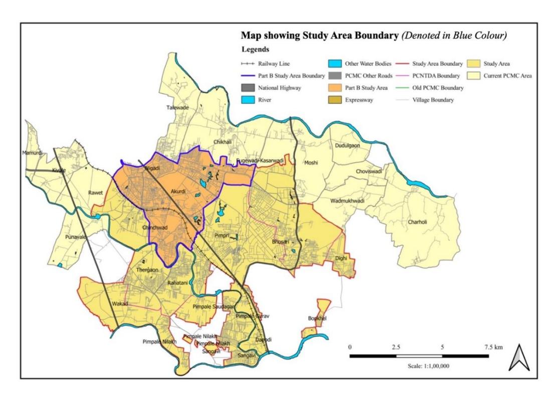
Figure 3. Map showing the study area in the blue boundaries. (Source: authors)
4. Selection criteria for identified slums
Even though the slums are spread all over the city, as shown in Figure 1, there is a larger concentration of slums in the Pimpri, Chinchwad, Akurdi, Bhosari, and Chikhali areas, as these have several significant commercial centers as well as major manufacturing industries. The urban poor tend to reside near these workplaces illegally, concentrated largely on public reservation lands. Hence, these slums all possess different morphologies in terms of density, built mass, characteristics, availability of services, etc. There were 37 slums within the study area of 22.95 km2 , as shown in Figure 3, out of which 26 were notified while eleven were non-notified. However, only twelve notified slum plots have been shortlisted for this research purpose. Shortlisting the twelve representative slums, the population density, notification period, plot area, accessibility, availability of infrastructure, and percentage of encroachment were considered as the major selection criteria.
Also, the area chosen for the case study covers a broad section of the city, including slums in the core area, urban area, and fringe area. The slum sites were marked considering the records available from the ULB government, as shown in Figure 4. Accordingly, the primary and secondary data were collected as per the needs of the framework.
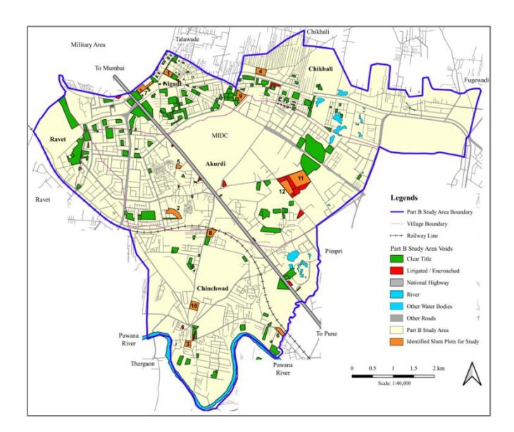
Figure 4. Map showing selected slum locations in the study area. (Source: authors)
Research Methodology
The main aim of this study was to find grey areas in the prevalent decision making in the site selection process for the redevelopment of slums or rehabilitation of the urban poor. It also establishes the need for the analysis of the sites based on selected parameters and decides their priority by scientifically weighing and ranking the scores. The ranking of these sites, which are urban voids, will give a clear direction for the decision makers, not only for the selection of sites but also for a logical allocation of funds, human resources, and government capacity.
This section gives a detailed idea about the selection of appropriate techniques in combination to get the desired results from a scientific, unbiased, and logical decision making process in slum site selection. It also provides the stepwise approach followed to derive the prioritization for slum site redevelopment.
1. Hybrid MADM model
The prioritization model for the selection of the most suitable slum sites for redevelopment purposes is based on criteria and their parameters, selected through Subject Matter Experts (SMEs). This prioritization model is a combination of assigning weights and deciding potentialbased ranking. Hence, it is pertinent to have a hybrid multi-attribute decision making (MADM) model that can consider several attributes for the final decision making. Our exploration suggested several combinations like AHP-TOPSIS, AHP-VIKOR, ENTROPY-TOPSIS, AHP PROMETHEE, AHP-MIVES, ENTROPY-VIKOR, etc. (Anojkumar et al., 2014; Jato-Espino et al., 2014; Lee & Chang, 2018; Stojčić et al., 2019). These combinations were reviewed while broadly considering their benefits, time required for the process, complexities considered, and type of results.
Finally, a combination of the Shannon's entropy and TOPSIS techniques was selected for this research, as it takes into consideration the degree of uncertainty or unpredictability in the data while measuring the weights of criteria (Hwang & Yoon, 1981; Shannon, 1948). This combination produces more reliable and accurate findings by reducing the subjectivity and uncertainty of the objective weights. As a result, several researchers have widely used this hybrid model for selection processes in the domain of mine safety evaluation (Yue, 2011), market segment selection (Duong & Thao, 2021), selection of sustainable materials (Reddy et al., 2022), selection of human resources (Yue, 2011), and integrated decision making for Covid-19 patients (Albahri et al., 2021) etc.
2. Shannon's entropy method
Shannon's entropy method is a quantitative method that can be used to determine the weights of criteria in decision making problems. The method involves calculating the entropy of each criterion, which may represent the degree of uncertainty or variability in the data for that criterion. It computes the weight based on the evaluation item's inherent quantity of information. The entropy values are then used to calculate the weights of the criteria, with higher weights assigned to criteria with lower entropy values (Shannon, 1948). This method is particularly useful when there are multiple criteria to consider and when the criteria are not equally important. It avoids deviations in deciding objective weights that may arise through the Analytical Hierarchy Process (AHP) and Delphi techniques (Li et al., 2011). However, this method can be used only for weight determination and thus has limited problem-solving capacity independently (Mou et al., 2020).
3. The TOPSIS method
The Technique of Order Preference Similarity to the Ideal Solution (TOPSIS) was developed by Hwang and Yoon in 1981(Hwang & Yoon, 1981). It is a widely used simple and programmable MADM technique that considers multiple attributes at a given time to obtain prioritization scores for all alternatives and rank them on their similarity to the ideal solution. The ideal solution is defined as the solution that maximizes the benefits and minimizes the costs of the decision problem. The simplicity of the process, the moderate computational time required, the stability of the results, and its ability to produce an indisputable preference order make the method more advantageous over several other methods (Chakraborty, 2011; Iç, 2012). As the method is based on Euclidean distance, positive or negative values do not influence the calculations. The method works better when indicators of alternatives do not vary much, as extreme deviation from ideal values can strongly influence the results (Siksnelyte-Butkiene et al., 2020).
Therefore, to get the maximum benefits in the decision-making process, the integration of the Shannon's entropy and TOPSIS methods was considered for this research.
4. Final six-Step methodology
To achieve the target objectives, the following six-step methodology was adopted:
- Step 1: Identify the criteria and parameters for evaluation.
- Step 2: Collect relevant primary and secondary data.
- Step 3: Derive the entropy weights.
- Step 4: Create a weighted normalized decision matrix for TOPSIS using the entropy weights.
- Step 5: Estimate the positive and negative scores in TOPSIS.
- Step 6: Prioritize the sites by calculating a relative proximity index and ranking the results.
Mathematical Model
This section provides the stepwise rational approach using a hybrid MADM method.
- 1. Shannon's entropy method for weight calculation
- (a) The entropy \(e_j\) of a set of normalized data \(P_{ij}\) for all j (j = 1 to k attributes and l = 1 to nalternatives) is calculated using the following formula:
\[e_j = -K \sum_{i=1}^n (P_{ij} * ln P_{ij})\]
(b) K is the constant given by
\[K = 1/lnN\]
K=1/lnN \(0 < e_i < 1\) K remains the same for all \(e_i\)
(c) Degree of divergence is calculated using
\[D_i = 1 - e_i\]
(d) Finally, the weights are calculated using
\[w_j = dj / \sum_{j=1}^n dj)\]
- 2. TOPSIS Method for priority index calculation and preference ranking
- (e) Standardized decision matrix A is constructed for comprehensive assessment questions with n evaluation units and m evaluation indexes, its decision matrix (A) and construction of normalized matrix (R).
\[\text{[rumus tidak dapat ditampilkan dengan baik — lihat PDF asli]}\]
Rij = xij / \[(\Sigma x2ij)\], for i = 1, ..., m; j = 1, ..., n.
(f) Weighted normalized decision matrix (V) is constructed using weights derived from Shannon's entropy model using
\[Vij=wj * Rij, i= 1, 2,...,n, j= 1,2,...m.\]
(g) The positive ideal solution (A+) and the negative ideal solution (A-) are determined using the following formula:
\[A^{+} = \{(\max_{i} v_{ij} | j \in J), (\min_{i} v_{ij} | j \in J) | i = 1, 2, ...n\}\] \[= \{(\min_{i} v_{ij} | j \in J), (\max_{i} v_{ij} | j \in J) | i = 1, 2, ...n\}\] \[= \{(\min_{i} v_{ij} | j \in J), (\max_{i} v_{ij} | j \in J) | i = 1, 2, ...n\}\] \[= \{(\min_{i} v_{ij} | j \in J), (\max_{i} v_{ij} | j \in J) | i = 1, 2, ...n\}\] \[\text{[rumus tidak dapat ditampilkan dengan baik — lihat PDF asli]}\]
- (h) The separation measures (Si+) from the positive ideal solution are calculated for each alternative using the following formula:
- (i) The separation measures (Si-) from the negative ideal solution are calculated for each alternative using the following formula:
\[S_{i}^{+} = \sqrt{\sum_{j=1}^{n} \left(v_{ij} - v_{j}^{+}\right)^{2}} \qquad i = 1, 2, ..., m\] \[S_{i}^{-} = \sqrt{\sum_{j=1}^{n} \left(v_{ij} - v_{j}^{-}\right)^{2}} \qquad i = 1, 2, ..., m\]
(j) The relative closeness coefficient (Ci) is calculated of each alternative to the ideal solution:
\[C_{i}^{*} = \frac{S_{i}}{(S_{i}^{+} + S_{i}^{-})}, \quad 0 < C_{i}^{*} < 1, \quad i = 1, 2, ..., m\] \[C_{i}^{*} = 1 \quad \text{if} \quad A_{i} = A^{+}\] \[C_{i}^{*} = 0 \quad \text{if} \quad A_{i} = A^{-}\]
(k) Finally, the priority of the alternatives is ranked in descending order of \(c_i\).
Data Processing
This research attempted to provide a comprehensive assessment framework for slum selection resulting from the derivation of weights and their prioritization. Furthermore, it considers the physical, infrastructural, legal, and environmental objective factors that are crucial in deciding the priority holistically. The assessment criteria and parameters for the slum plots (Table 1) were identified through a literature review and finalized through subject matter experts (SMEs) with a structured opinion survey. About twelve experts were identified from several relevant sectors, including the government, private sector, academia, and research groups for a holistic opinion.
Table 1. List of criteria and parameters finalized for the study through SME's. (Source: authors)
| Criteria | Criteria Code | Parameter | Parameter Code |
|---|---|---|---|
| L1 | Population Density (per km²) | PD | |
| Legal Parameters | L2 | Notification Period (in months | NP |
| 1 at affecters | L3 | Land Value (Rs. per foot2) | LV |
| T1 | Plot Area (in km²) | PA | |
| T | T2 | Plot Shape | PS |
| Topography | T3 | Soil Type | ST |
| T4 | Plot Gradient | PG | |
| II | Road Accessibility | RA | |
| Infrastructure | I2 | Availability of Physical Infrastructure | PI |
| I3 | Building Density & Structural Stability | DS | |
| P1 | Proximity to the Public Transport | PT | |
| Proximity | P2 | Proximity to the Social Infrastructure | SI |
| P3 | Proximity to the Economic Centres | EC | |
| Diala | R1 | Degree of Encroachment of Public Reservation (%) | DE |
| Risks | R2 | Degree of Risk of Natural Disaster of the Site | ND |
However, as the notified slum plots belonged to the government, it has been their responsibility to provide affordable housing with land tenure under social welfare to the urban poor. Also, the socio-economic structures and behavioral issues of the inhabitants have been very dynamic and complex, hence these parameters were excluded by the experts.
The structured opinions were taken on a Likert scale from 5 to 1, with 5 = 'Most Important Parameter', 4 = 'Important Parameter', 3 = 'Neutral Parameter', 2 = 'Least Important Parameter' and 1 = 'Unimportant Parameter'. The quantitative analysis of all SMEs opinions was done using the weighted mean method and standard deviation. Above is the list of criteria and respective parameters finalized through this process (Table 1).
Results & Discussion
As mentioned in the research methodology section, the desired results were achieved through a six-step methodology discussed in detail as follows:
Step 1: Identify the criteria and parameters for evaluation: The criteria and parameters mentioned in Table 1 used for evaluation of the different slum sites were identified based on the literature review and the structured opinion of the SMEs. These parameters helped us to understand the underlying factors required in the decision making process.
Step 2: Collect relevant primary and secondary data: Table 2 mentions the data collected through physical surveys, site visits, and data from the urban local body (ULB). This was of the utmost importance in helping to understand the real-time scenario, the status of the slums, and problems in phase-wise slum plot selection.
Step 3: Derive the entropy weights: The data from Table 2 was analyzed using Shannon's entropy method to derive the weights for each parameter. Using the mathematical model given in the research methodology section, the following results were derived. Table 3 shows the final weights (Wj) for each parameter. The cumulative entropy weight for Legal Particulars (L1 + L2 + L3) was 0.2318, for Topography (T1 + T2 + T3 + T4) it was 0.3924, for Infrastructure (I1 + I2 + I3) it was 0.1610, for Proximity (P1 + P2 + P3) it was 0.1547, and for Risks (R1 + R2) it was 0.0601.
Thus, the highest weights were derived for the Topography Criteria, the second highest for the Legal Particulars, the third highest for the Infrastructure Criteria, and the fourth highest for the Proximity Criteria. The lowest weight was derived for the Risk Criteria. Furthermore, it clearly indicates that the parameters Plot Area (T1 = 0.2069), Land Value (L3 = 0.1189), Building Density and Structural Stability (I3 = 0.0779), Plot Shape (T2 = 0.0776), and Population Density (L1= 0.0676) were the five top major factors dominating the decision making.
The entropy matrix also conveys that the Notification Period (L2 = 0.0453), Degree of Risk of Natural Disaster of the site (R2 = 0.0397), Availability Physical Infrastructure (I2 = 0.0369), Proximity to Social Infrastructure (P2 = 0.0362) and Degree of Encroachment of Public Reservation (R1 = 0.0204)) were also important but at the lowest order in deciding the priority of redevelopment.
Step 4: Create a weighted normalized decision matrix: The weighted normalized matrix was determined after multiplying the entropy weights derived in Step 3 and the normalized decision matrix derived through TOPSIS as mentioned in Table 4.
Table 2. List of data sets for identified urban void slum plots. (Source: authors)
| Risks | Degree of Risk of Natural Disaster of the site | R2 | ND | 2 (High Risk) | 4 (Low Risk) | 4 (Low Risk) | 3 (Moderate Risk | 5 (Very Low Risk) | 2 (High Risk) | 4 (Low Risk) | 5 (Very Low Risk) | 4 (Low Risk) | 4 (Low Risk) | 4 (Low Risk) | 3 (Moderate Risk | |
|---|---|---|---|---|---|---|---|---|---|---|---|---|---|---|---|---|
| Ri | Degree of Encro. of public Reservation (%) | RI | DE | 50 | 80 | 06 | 82 | 70 | 100 | 09 | 75 | 100 | 08 | 100 | 82 | |
| Proximity to Eco. Centers | P3 | EC | 2 (Poor) | 5 (Very Good) | 3 (Moderate) | 5 (Very Good) | 3 (Moderate) | 5 (Very Good) | 2 (Poor) | 5 (Very Good) | 5 (Very Good) | 4 (Good) | 5 (Very Good) | 5 (Very Good) | ||
| Proximity | Proximity to Social Infra. | P2 | SI | 3 (Moderate) | 3 (Moderate) | 3 (Moderate) | 2 (Poor) | 3 (Moderate) | 2 (Poor) | 3 (Moderate) | 4 (Good) | 5 (Very Good) | 4 (Good) | 4 (Good) | 3 (Moderate) | |
| Proximity to the Public Transport. | PI | PT | 4 (Good) | 3 (Moderate) | 1 (Very Poor) | 4 (Good) | 2 (Poor) | 3 (Moderate) | 4 (Good) | 5 (Very Good) | 4 (Good) | 3 (Moderate) | 5 (Very Good) | 4 (Good) | ||
| Building Density and Structural Stability | 13 | DS | 2 (Poor) | 5 (Very Good) | 3 (Moderate) | 4 (Good) | 3 (Moderate) | 2 (Poor) | 3 (Moderate) | 4 (Good) | 4 (Good) | 1 (Very Poor) | 4 (Good) | 3 (Moderate) | ||
| Void Plots | Infrastructure | Availability Physical Infrastructure | 12 | PI | 2 (Poor Quality) | 4 (Good Quality) | 3 (Moderate Quality) | 4 (Good Quality) | 3 (Moderate Quality) | 4 (Good Quality) | 2 (Poor Quality) | 5 (Very Good Quality) | 3 (Moderate Quality) | 3 (Moderate Quality) | 4 (Good Quality) | 4 (Good Quality) |
| Data Set for identified Slum Void Plots | 4 | Road Accessibility | П | RA | 4 (Good Accessibility) | 3 (Moderate Accessibility) | 2 (Poor Accessibility) | 4 (Good Accessibility) | 2 (Poor Accessibility) | 2 (Poor Accessibility) | 4 (Good Accessibility) | 5 (Very Good Accessibility) | 4 (Good Accessibility) | 3 (Moderate Accessibility) | 4 (Good Accessibility) | 4 (Good Accessibility) |
| Set for iden | Plot Gradient | T4 | PG | 3 (Moderate Slope) | 5 (Highly Flat) | 4 (Flat) | 4 (Flat) | 2 (High Slope) | 2 (High Slope) | 3 (Moderate Slope) | 5 (Highly Flat) | 4 (Flat) | 5 (Highly Flat) | 5 (Highly Flat) | 2 (High Slope) | |
| Data | Topography | Soil Type | T3 | ST | 2 (Less Strengthy) | 4 (Strengthy) | 5 (Highly Strengthy) | 3 (Moderately Strengthy) | 5 (Highly Strengthy) | 2 (Less Strengthy) | 4 (Strengthy) | 5 (Highly Strengthy) | 5 (Highly Strengthy) | 4 (Strengthy) | 4 (Strengthy) | 3 (Moderately Strengthy) |
| Topo | Plot Shape | 7.2 | PS | 3 (Moderately Developable) | 4 (Developable) | 3 (Moderately Developable) | 5 (Highly Developable) | 2 (Less Developable) | 1 (Not Developable) | 3 (Moderately Developable) | 4 (Developable) | 4 (Developable) | 4 (Developable) | 5 (Highly Developable) | 2 (Less Developable) | |
| Plot Area (Sq. M.) | TI | PA | 14581 | 31634 | 11267 | 16930 | 8581 | 10432 | 12785 | 16280 | 38145 | 19335 | 62478 | 31489 | ||
| Land Value (Sq. Ft.) | T3 | LV | 780 | 2255 | 756 | 1915 | 845 | 1195 | 790 | 2776 | 999 | 1452 | 1775 | 1359 | ||
| Legal Particulars | Notification Period (In Months) | 1.2 | NP | 40 | 105 | 89 | 124 | 72 | 96 | 54 | 112 | 102 | 96 | 108 | 100 | |
| Leg | Population Density (Sq. Km.) | ΓI | PD | 7895 | 12220 | 8621 | 15295 | 7845 | 9430 | 9855 | 11450 | 16380 | 10560 | 24350 | 14750 | |
| Criteria | Para- meters | Plot 1 | Plot 2 | Plot 3 | Plot 4 | Plot 5 | Plot 6 | Plot 7 | Plot 8 | Plot 9 | Plot 10 | Plot 11 | Plot 12 |
Table 3. Final Weight Derivation. (Source: authors)
| Pij: Normalized Decision Matrix | |||||||||||||||
|---|---|---|---|---|---|---|---|---|---|---|---|---|---|---|---|
| Criteria | Legal Particulars | Topography | Infrastructure | Proximity | Risks | ||||||||||
| Parameters | PD | NP | LV | PA | PS | ST | PG | RA | PI | DS | PT | SI | EC | DE | ND |
| Plot 1 | 0.0531 | 0.0371 | 0.0471 | 0.0532 | 0.0750 | 0.0435 | 0.0682 | 0.0976 | 0.0488 | 0.0513 | 0.0952 | 0.0769 | 0.0408 | 0.0513 | 0.0455 |
| Plot 2 | 0.0822 | 0.0975 | 0.1362 | 0.1155 | 0.1000 | 0.0870 | 0.1136 | 0.0732 | 0.0976 | 0.1282 | 0.0714 | 0.0769 | 0.1020 | 0.0821 | 0.0909 |
| Plot 3 | 0.0580 | 0.0631 | 0.0456 | 0.0411 | 0.0750 | 0.1087 | 0.0909 | 0.0488 | 0.0732 | 0.0769 | 0.0238 | 0.0769 | 0.0612 | 0.0923 | 0.0909 |
| Plot 4 | 0.1029 | 0.1151 | 0.1156 | 0.0618 | 0.1250 | 0.0652 | 0.0909 | 0.0976 | 0.0976 | 0.1026 | 0.0952 | 0.0513 | 0.1020 | 0.0872 | 0.0682 |
| Plot 5 | 0.0528 | 0.0669 | 0.0510 | 0.0313 | 0.0500 | 0.1087 | 0.0455 | 0.0488 | 0.0732 | 0.0769 | 0.0476 | 0.0769 | 0.0612 | 0.0718 | 0.1136 |
| Plot 6 | 0.0634 | 0.0891 | 0.0722 | 0.0381 | 0.0250 | 0.0435 | 0.0455 | 0.0488 | 0.0976 | 0.0513 | 0.0714 | 0.0513 | 0.1020 | 0.1026 | 0.0455 |
| Plot 7 | 0.0663 | 0.0501 | 0.0477 | 0.0467 | 0.0750 | 0.0870 | 0.0682 | 0.0976 | 0.0488 | 0.0769 | 0.0952 | 0.0769 | 0.0408 | 0.0615 | 0.0909 |
| Plot 8 | 0.0770 | 0.1040 | 0.1676 | 0.0594 | 0.1000 | 0.1087 | 0.1136 | 0.1220 | 0.1220 | 0.1026 | 0.1190 | 0.1026 | 0.1020 | 0.0769 | 0.1136 |
| Plot 9 | 0.1102 | 0.0947 | 0.0400 | 0.1392 | 0.1000 | 0.1087 | 0.0909 | 0.0976 | 0.0732 | 0.1282 | 0.0952 | 0.1282 | 0.1020 | 0.1026 | 0.0909 |
| Plot 10 | 0.0710 | 0.0891 | 0.0877 | 0.0706 | 0.1000 | 0.0870 | 0.1136 | 0.0732 | 0.0732 | 0.0256 | 0.0714 | 0.1026 | 0.0816 | 0.0821 | 0.0909 |
| Plot 11 | 0.1638 | 0.1003 | 0.1072 | 0.2281 | 0.1250 | 0.0870 | 0.1136 | 0.0976 | 0.0976 | 0.1026 | 0.1190 | 0.1026 | 0.1020 | 0.1026 | 0.0909 |
| Plot 12 | 0.0992 | 0.0929 | 0.0821 | 0.1149 | 0.0500 | 0.0652 | 0.0455 | 0.0976 | 0.0976 | 0.0769 | 0.0952 | 0.0769 | 0.1020 | 0.0872 | 0.0682 |
| Pij * ln Pij | |||||||||||||||
| Criteria | Legal Particulars | Topography | Infrastructure | Proximity | Risks | ||||||||||
| Parameters | PD | NP | LV | PA | PS | ST | PG | RA | PI | DS | PT | SI | EC | DE | ND |
| Plot 1 | -0.1559 | -0.1223 | -0.1439 | -0.1561 | -0.1943 | -0.1363 | -0.1831 | -0.2271 | -0.1473 | -0.1523 | -0.2239 | -0.1973 | -0.1306 | -0.1523 | -0.1405 |
| Plot 2 | -0.2054 | -0.2270 | -0.2715 | -0.2493 | -0.2303 | -0.2124 | -0.2471 | -0.1913 | -0.2271 | -0.2633 | -0.1885 | -0.1973 | -0.2329 | -0.2052 | -0.2180 |
| Plot 3 | -0.1651 | -0.1744 | -0.1409 | -0.1312 | -0.1943 | -0.2412 | -0.2180 | -0.1473 | -0.1913 | -0.1973 | -0.0890 | -0.1973 | -0.1710 | -0.2199 | -0.2180 |
| Plot 4 | -0.2340 | -0.2489 | -0.2495 | -0.1720 | -0.2599 | -0.1780 | -0.2180 | -0.2271 | -0.2271 | -0.2336 | -0.2239 | -0.1523 | -0.2329 | -0.2127 | -0.1831 |
| Plot 5 | -0.1552 | -0.1809 | -0.1518 | -0.1085 | -0.1498 | -0.2412 | -0.1405 | -0.1473 | -0.1913 | -0.1973 | -0.1450 | -0.1973 | -0.1710 | -0.1891 | -0.2471 |
| Plot 6 | -0.1749 | -0.2155 | -0.1897 | -0.1245 | -0.0922 | -0.1363 | -0.1405 | -0.1473 | -0.2271 | -0.1523 | -0.1885 | -0.1523 | -0.2329 | -0.2336 | -0.1405 |
| Plot 7 | -0.1799 | -0.1501 | -0.1451 | -0.1430 | -0.1943 | -0.2124 | -0.1831 | -0.2271 | -0.1473 | -0.1973 | -0.2239 | -0.1973 | -0.1306 | -0.1716 | -0.2180 |
| Plot 8 | -0.1975 | -0.2354 | -0.2994 | -0.1678 | -0.2303 | -0.2412 | -0.2471 | -0.2566 | -0.2566 | -0.2336 | -0.2534 | -0.2336 | -0.2329 | -0.1973 | -0.2471 |
| Plot 9 | -0.2430 | -0.2232 | -0.1288 | -0.2745 | -0.2303 | -0.2412 | -0.2180 | -0.2271 | -0.1913 | -0.2633 | -0.2239 | -0.2633 | -0.2329 | -0.2336 | -0.2180 |
| Plot 10 | -0.1879 | -0.2155 | -0.2134 | -0.1871 | -0.2303 | -0.2124 | -0.2471 | -0.1913 | -0.1913 | -0.0939 | -0.1885 | -0.2336 | -0.2045 | -0.2052 | -0.2180 |
| Plot 11 | -0.2963 | -0.2306 | -0.2394 | -0.3371 | -0.2599 | -0.2124 | -0.2471 | -0.2271 | -0.2271 | -0.2336 | -0.2534 | -0.2336 | -0.2329 | -0.2336 | -0.2180 |
| Plot 12 | -0.2292 | -0.2207 | -0.2052 | -0.2487 | -0.1498 | -0.1780 | -0.1405 | -0.2271 | -0.2271 | -0.1973 | -0.2239 | -0.1973 | -0.2329 | -0.2127 | -0.1831 |
| Sum | -2.4244 | -2.4444 | -2.3786 | -2.2999 | -2.4155 | -2.4431 | -2.4302 | -2.4436 | -2.4519 | -2.4152 | -2.4259 | -2.4525 | -2.4379 | -2.4667 | -2.4494 |
| Final Weights | |||||||||||||||
| 1-eij eij | 0.9757 0.0243 | 0.9837 0.0163 | 0.9572 0.0428 | 0.9255 0.0745 | 0.0279 0.9721 | 0.9832 0.0168 | 0.9780 0.0220 | 0.9834 0.0166 | 0.9867 0.0133 | 0.9720 0.0280 | 0.9763 0.0237 | 0.9870 0.0130 | 0.0189 0.9811 | 0.9927 0.0073 | 0.9857 0.0143 |
| wj | 0.0676 | 0.0453 | 0.1189 | 0.2069 | 0.0776 | 0.0467 | 0.0612 | 0.0462 | 0.0369 | 0.0779 | 0.0660 | 0.0362 | 0.0525 | 0.0204 | 0.0397 |
Table 4. Table showing positive and negative ideal solutions. (Source: authors)
Rij: Normalized Decision Matrix
| wy. two | ng. Tolmantea Decision mail a | MINITED IN | |||||||||||||
|---|---|---|---|---|---|---|---|---|---|---|---|---|---|---|---|
| Criteria | \(\Gamma\epsilon\) | Legal Particulars | us | Topography | "aphy | ľ | nfrastructure | Proximity | Risks | ks | |||||
| Parameters | DD | NP | TN | PA | PS | ST | PG | RA | Id | DS | PT | IS | EC | DE | ND |
| Plot I | 0.1727 | 0.1242 | 0.1475 | 0.1540 | 0.2449 | 0.1451 | 0.2249 | 0.3255 | 0.1638 | 0.1672 | 0.3143 | 0.2582 | 0.1358 | 0.1746 | 0.1525 |
| Plot 2 | 0.2674 | 0.3260 | 0.4265 | 0.3342 | 0.3266 | 0.2902 | 0.3748 | 0.2441 | 0.3277 | 0.4181 | 0.2357 | 0.2582 | 0.3394 | 0.2794 | 0.3050 |
| Plot 3 | 0.1886 | 0.1430 | 0.1190 | 0.2449 | 0.3627 | 0.2998 | 0.1628 | 0.2458 | 0.2509 | 0.0786 | 0.2582 | 0.2037 | 0.3143 | 0.3050 | |
| Plot 4 | 0.3346 | 0.3849 | 0.3622 | 0.1788 | 0.4082 | 0.2176 | 0.2998 | 0.3255 | 0.3277 | 0.3345 | 0.3143 | 0.1721 | 0.3394 | 0.2969 | 0.2287 |
| Plot 5 | 0.1716 | 0.1598 | 9060.0 | 0.1633 | 0.3627 | 0.1499 | 0.1628 | 0.2458 | 0.2509 | 0.1571 | 0.2582 | 0.2037 | 0.2445 | 0.3812 | |
| Plot 6 | 0.2063 | 0.2980 0.2260 | 0.2260 | 0.1102 | 0.0816 | 0.1451 | 0.1499 | 0.1628 | 0.3277 | 0.1672 | 0.2357 | 0.1721 | 0.3394 | 0.3493 | 0.1525 |
| Plot 7 | 0.2156 | 0.1676 | 0.1494 | 0.1351 | 0.2449 | 0.2902 | 0.2249 | 0.3255 | 0.1638 | 0.2509 | 0.3143 | 0.2582 | 0.1358 | 0.2096 | 0.3050 |
| Plot 8 | 0.2505 | 0.3477 | 0.5251 | 0.1720 | 0.3266 | 0.3627 | 0.3748 | 0.4069 | 0.4096 | 0.3345 | 0.3928 | 0.3443 | 0.3394 | 0.2620 | 0.3812 |
| Plot 9 | 0.3584 | 0.3166 | 0.1254 | 0.4029 | 0.3266 | 0.3627 | 0.2998 | 0.3255 | 0.2458 | 0.4181 | 0.3143 | 0.4303 | 0.3394 | 0.3493 | 0.3050 |
| Plot 10 | 0.2310 | 0.2980 | 0.2746 | 0.2042 | 0.3266 | 0.2902 | 0.3748 | 0.2441 | 0.2458 | 0.0836 | 0.2357 | 0.3443 | 0.2715 | 0.2794 | 0.3050 |
| Plot 11 | 0.5328 | 0.3353 | 0.3357 | 0.6600 | 0.4082 | 0.2902 | 0.3748 | 0.3255 | 0.3277 | 0.3345 | 0.3928 | 0.3443 | 0.3394 | 0.3493 | 0.3050 |
| Plot 12 | 0.3227 | 0.3104 | 0.2571 | 0.3326 | 0.1633 | 0.2176 | 0.1499 | 0.3255 | 0.3277 | 0.2509 | 0.3143 | 0.2582 | 0.3394 | 0.2969 | 0.2287 |
| Criteria | Legal Particulars | Topography | Infrastructure | Proximity | Risks | ||||||||||
|---|---|---|---|---|---|---|---|---|---|---|---|---|---|---|---|
| Parameters | PD | NP | LV | PA | PS | ST | PG | RA | PI | DS | PT | SI | EC | DE | ND |
| Plot 1 | 0.1727 | 0.1242 | 0.1475 | 0.1540 | 0.2449 | 0.1451 | 0.2249 | 0.3255 | 0.1638 | 0.1672 | 0.3143 | 0.2582 | 0.1358 | 0.1746 | 0.1525 |
| Plot 2 | 0.2674 | 0.3260 | 0.4265 | 0.3342 | 0.3266 | 0.2902 | 0.3748 | 0.2441 | 0.3277 | 0.4181 | 0.2357 | 0.2582 | 0.3394 | 0.2794 | 0.3050 |
| Plot 3 | 0.1886 | 0.2111 | 0.1430 | 0.1190 | 0.2449 | 0.3627 | 0.2998 | 0.1628 | 0.2458 | 0.2509 | 0.0786 | 0.2582 | 0.2037 | 0.3143 | 0.3050 |
| Plot 4 | 0.3346 | 0.3849 | 0.3622 | 0.1788 | 0.4082 | 0.2176 | 0.2998 | 0.3255 | 0.3277 | 0.3345 | 0.3143 | 0.1721 | 0.3394 | 0.2969 | 0.2287 |
| Plot 5 | 0.1716 | 0.2235 | 0.1598 | 0.0906 | 0.1633 | 0.3627 | 0.1499 | 0.1628 | 0.2458 | 0.2509 | 0.1571 | 0.2582 | 0.2037 | 0.2445 | 0.3812 |
| Plot 6 | 0.2063 | 0.2980 | 0.2260 | 0.1102 | 0.0816 | 0.1451 | 0.1499 | 0.1628 | 0.3277 | 0.1672 | 0.2357 | 0.1721 | 0.3394 | 0.3493 | 0.1525 |
| Plot 7 | 0.2156 | 0.1676 | 0.1494 | 0.1351 | 0.2449 | 0.2902 | 0.2249 | 0.3255 | 0.1638 | 0.2509 | 0.3143 | 0.2582 | 0.1358 | 0.2096 | 0.3050 |
| Plot 8 | 0.2505 | 0.3477 | 0.5251 | 0.1720 | 0.3266 | 0.3627 | 0.3748 | 0.4069 | 0.4096 | 0.3345 | 0.3928 | 0.3443 | 0.3394 | 0.2620 | 0.3812 |
| Plot 9 | 0.3584 | 0.3166 | 0.1254 | 0.4029 | 0.3266 | 0.3627 | 0.2998 | 0.3255 | 0.2458 | 0.4181 | 0.3143 | 0.4303 | 0.3394 | 0.3493 | 0.3050 |
| Plot 10 | 0.2310 | 0.2980 | 0.2746 | 0.2042 | 0.3266 | 0.2902 | 0.3748 | 0.2441 | 0.2458 | 0.0836 | 0.2357 | 0.3443 | 0.2715 | 0.2794 | 0.3050 |
| Plot 11 | 0.5328 | 0.3353 | 0.3357 | 0.6600 | 0.4082 | 0.2902 | 0.3748 | 0.3255 | 0.3277 | 0.3345 | 0.3928 | 0.3443 | 0.3394 | 0.3493 | 0.3050 |
| Plot 12 | 0.3227 | 0.3104 | 0.2571 | 0.3326 | 0.1633 | 0.2176 | 0.1499 | 0.3255 | 0.3277 | 0.2509 | 0.3143 | 0.2582 | 0.3394 | 0.2969 | 0.2287 |
| Vij: Weighted Normalized Matrix | |||||||||||||||
| Criteria | Legal Particulars | Topography | Infrastructure | Proximity | Risks | ||||||||||
| Parameters | PD | NP | LV | PA | PS | ST | PG | RA | PI | DS | PT | SI | EC | DE | ND |
| Plot 1 | 0.0117 | 0.0056 | 0.0175 | 0.0319 | 0.0190 | 0.0068 | 0.0138 | 0.0150 | 0.0060 | 0.0130 | 0.0207 | 0.0093 | 0.0071 | 0.0036 | 0.0061 |
| Plot 2 | 0.0181 | 0.0148 | 0.0507 | 0.0691 | 0.0253 | 0.0136 | 0.0229 | 0.0113 | 0.0121 | 0.0326 | 0.0155 | 0.0093 | 0.0178 | 0.0057 | 0.0121 |
| Plot 3 | 0.0128 | 0.0096 | 0.0170 | 0.0246 | 0.0190 | 0.0169 | 0.0183 | 0.0075 | 0.0091 | 0.0196 | 0.0052 | 0.0093 | 0.0107 | 0.0064 | 0.0121 |
| Plot 4 | 0.0226 | 0.0174 | 0.0431 | 0.0370 | 0.0317 | 0.0102 | 0.0183 | 0.0150 | 0.0121 | 0.0261 | 0.0207 | 0.0062 | 0.0178 | 0.0061 | 0.0091 |
| Plot 5 | 0.0116 | 0.0101 | 0.0190 | 0.0188 | 0.0127 | 0.0169 | 0.0092 | 0.0075 | 0.0091 | 0.0196 | 0.0104 | 0.0093 | 0.0107 | 0.0050 | 0.0151 |
| Plot 6 | 0.0139 | 0.0135 | 0.0269 | 0.0228 | 0.0063 | 0.0068 | 0.0092 | 0.0075 | 0.0121 | 0.0130 | 0.0155 | 0.0062 | 0.0178 | 0.0071 | 0.0061 |
| Plot 7 | 0.0146 | 0.0076 | 0.0178 | 0.0279 | 0.0190 | 0.0136 | 0.0138 | 0.0150 | 0.0060 | 0.0196 | 0.0207 | 0.0093 | 0.0071 | 0.0043 | 0.0121 |
| Plot 8 | 0.0169 | 0.0158 | 0.0624 | 0.0356 | 0.0253 | 0.0169 | 0.0229 | 0.0188 | 0.0151 | 0.0261 | 0.0259 | 0.0125 | 0.0178 | 0.0053 | 0.0151 |
| Plot 9 | 0.0242 | 0.0143 | 0.0149 | 0.0834 | 0.0253 | 0.0169 | 0.0183 | 0.0150 | 0.0091 | 0.0326 | 0.0207 | 0.0156 | 0.0178 | 0.0071 | 0.0121 |
| Plot 10 | 0.0156 | 0.0135 | 0.0326 | 0.0423 | 0.0253 | 0.0136 | 0.0229 | 0.0113 | 0.0091 | 0.0065 | 0.0155 | 0.0125 | 0.0143 | 0.0057 | 0.0121 |
| Plot 11 | 0.0360 | 0.0152 | 0.0399 | 0.1366 | 0.0317 | 0.0136 | 0.0229 | 0.0150 | 0.0121 | 0.0261 | 0.0259 | 0.0125 | 0.0178 | 0.0071 | 0.0121 |
| Plot 12 | 0.0218 | 0.0141 | 0.0306 | 0.0688 | 0.0127 | 0.0102 | 0.0092 | 0.0150 | 0.0121 | 0.0196 | 0.0207 | 0.0093 | 0.0178 | 0.0061 | 0.0091 |
| Max Value | 0.0360 | 0.0174 | 0.0624 | 0.1366 | 0.0317 | 0.0169 | 0.0229 | 0.0188 | 0.0151 | 0.0326 | 0.0259 | 0.0156 | 0.0178 | 0.0071 | 0.0151 |
| Min Value | 0.0116 | 0.0056 | 0.0149 | 0.0188 | 0.0063 | 0.0068 | 0.0092 | 0.0075 | 0.0060 | 0.0065 | 0.0052 | 0.0062 | 0.0071 | 0.0036 | 0.0061 |
| B / NB | B | NB | B | B | B | B | NB | B | B | B | B | B | B | NB | NB |
| A+ | 0.0360 | 0.0056 | 0.0624 | 0.1366 | 0.0317 | 0.0169 | 0.0092 | 0.0188 | 0.0151 | 0.0326 | 0.0259 | 0.0156 | 0.0178 | 0.0036 | 0.0061 |
| A- | 0.0116 | 0.0174 | 0.0149 | 0.0188 | 0.0063 | 0.0068 | 0.0229 | 0.0075 | 0.0060 | 0.0065 | 0.0052 | 0.0062 | 0.0071 | 0.0071 | 0.0151 |
Step 5: Estimate the positive and negative ideal solutions in TOPSIS: Table 4 also shows the positive ideal solution (A+) and negative ideal solution (A-) scores for each slum plot alternative as estimated through TOPSIS. In this process, both the Beneficial(B) and Non-Beneficial (NB) parameters were decided and, accordingly, the scores were established.
Step 6: Prioritize the slum sites: The separation measure (Si+) from the positive ideal solutions and separation measure (Si-) from the negative ideal solutions scores were derived using the scores from Step 5. These scores assisted in establishing the relative closeness coefficient Ci of each alternative to the positive and negative ideal solutions. The systematic ranking of all alternative plots was done using this coefficient mentioned in Table 5. All the ranks were then arranged in descending order to decide the prioritization of slum plots for redevelopment.
Table 5. Table showing relative closeness coefficient and final ranking. (Source: authors)
| Ci = Relative Closeness Coefficient | ||||
|---|---|---|---|---|
| Slum Plot No. | Si+ | Si- | Ci | Ranks |
| Plot 1 | 0.1205 | 0.0318 | 0.2087 | 8 |
| Plot 2 | 0.0747 | 0.0725 | 0.4923 | 3 |
| Plot 3 | 0.1276 | 0.0245 | 0.1608 | 11 |
| Plot 4 | 0.1046 | 0.0528 | 0.3357 | 6 |
| Plot 5 | 0.1323 | 0.0252 | 0.1601 | 12 |
| Plot 6 | 0.1274 | 0.0274 | 0.1772 | 10 |
| Plot 7 | 0.1222 | 0.0314 | 0.2043 | 9 |
| Plot 8 | 0.1050 | 0.0649 | 0.3820 | 5 |
| Plot 9 | 0.0745 | 0.0776 | 0.5103 | 2 |
| Plot 10 | 0.1070 | 0.0392 | 0.2683 | 7 |
| Plot 11 | 0.0304 | 0.1298 | 0.8104 | 1 |
| Plot 12 | 0.0810 | 0.0614 | 0.4314 | 4 |
Prioritization of Alternatives in Descending Order
| Slum Plot No. | Ci* | Ranks |
|---|---|---|
| Plot 11 | 0.8104 | 1 |
| Plot 9 | 0.5103 | 2 |
| Plot 2 | 0.4923 | 3 |
| Plot 12 | 0.4314 | 4 |
| Plot 8 | 0.3820 | 5 |
| Plot 4 | 0.3357 | 6 |
| Plot 10 | 0.2683 | 7 |
| Plot 1 | 0.2087 | 8 |
| Plot 7 | 0.2043 | 9 |
| Plot 6 | 0.1772 | 10 |
| Plot 3 | 0.1608 | 11 |
| Plot 5 | 0.1601 | 12 |
Discussion
Overall, the results produced an analysis framework where physical, infrastructural, legal, and environmental objective factors were assessed for the redevelopment of slums, comprehensively covering context-specific qualitative and quantitative criteria and parameters. Although a lot of literature is available worldwide on addressing infrastructural, social, economic, and behavioral issues, limited attempts have been made to assess the potential of slums considering them as urban voids, which is a pertinent concern for the decision makers.
This research tried to fill this gap by providing an impartial and scientific mechanism by employing a hybrid MADM method. This method is robust enough to consider the degree of uncertainty or variability in the data for all criteria as it computes the entropy weight based on the evaluation item's inherent quantity of information. Additionally, the TOPSIS method is flexible enough to consider multiple attributes at a given time to obtain prioritization scores for all urban voids and rank them on their similarity to the ideal solution, thus maximizing the benefits.
Hence, the desired objectives of the study were achieved by the hybrid combination of Shannon's entropy and TOPSIS employed for the assessment of the development potential of urban voids as well as the provision of a methodical and scientific approach for their prioritization. Finally, the outcomes of the proposed method can be widely applied due to its inbuilt flexibility and adaptability.
Conclusions
Worldwide, especially in the Global South, the equitable supply of affordable housing has been a challenging affair for ULB governments. Changing governments, uneven devolution of funds and complex political agendas have adversely brought biases within the selection process of urban voids with slums for redevelopment. It has also undesirably affected the time taken for decision making and increased budgets enormously. Internationally, the approach to slum improvement has changed from slum clearance to slum redevelopment, however, this research also conveyed that it has changed the role of the government from a destroyer to an advisor, to a supplier, to a facilitator.
At the outset, the research attempted a way forward through a scientific, unbiased, justifiable, and legitimate process in the rightful selection of urban voids with slums, with a comprehensive analysis framework. For the decision makers who majorly have the role of supplier and facilitator, it has always been a challenge to logically select urban voids with slums. This genuine problem was addressed by the research with the application of a hybrid method of MADM, Shannon's entropy, and TOPSIS.
The precise and consistent results generated a prioritization of urban voids for redevelopment. The process ensures the decision makers about the legitimate allocation of funds and resources in the most effective and time-efficient manner, while eliminating the bias. Although the study comprehensively covered all area-specific parameters, it could be modified as per different contexts, while keeping the methodology intact. Additionally, the data was majorly collected from limited primary and secondary sources. Periodical data collection will give more accurate results. Further, this exercise could be extended for the prioritization of similar urban voids either according to ward, administrative zone, or city-wide, which can be easily done utilizing the appropriate data.
Finally, we hope that the derived streamlined framework will act as a tool in the overall process of poverty alleviation in accordance with the sustainable development goals (SDGs) while addressing the needs of economically weaker section (EWS) communities living in urban areas more democratically. Such exercises will empower the modus operandi intended for the upliftment of the urban poor, which is most significant in achieving integrated balanced urban development of cities in the Global South, especially in India.