
Introduction
Public transport plays a crucial role in fostering economic growth and development (Prchal, 2019), making the efficiency of public transport directly translate into urban policy planning. In principle, public transport can compete with private cars (Mattiolo et al., 2020). However, it should be noted that inefficient public transport will increase dependence on private cars, which is an undesirable phenomenon in cities. Therefore, it is crucial to determine the effectiveness of public transport and compare it to private cars, in order to identify further directions of the implemented transport policy in a given city.
In-vehicle time (IVT) is one of the fundamental parameters of a trip that determines the choice of a particular mode of transport. It is also an important parameter in modelling transport demand (Douglas and Wallis, 2013) and vehicle routing algorithms (Fleischmann, Gietz and Gnutzmann, 2004). The specificity of public transport (traveling on a planned route with stops at stations) results in its IVT being significantly higher compared to private car transport. Furthermore, to fully evaluate a trip, parameters such as access time to the vehicle and waiting time must also be considered in addition to IVT (Wardman, 2004). It should also be noted that people value access time and waiting time more than IVT. This situation has been observed both in the past (Quarmby, 1967; Daly and Zachary, 1975) and in present times (Wardman, 2001; Abrantes and Wardman, 2011). Access parameters are practically non-existent in personal transport, except for the situation of leaving the vehicle in a remote parking lot. Moreover, these parameters will differ depending on the passenger's transport behavior; in the case of public transport, their values are lower for planned trips and higher for spontaneous trips. However, public transport users can significantly minimize waiting time by planning their trip with a timetable in mind. Good accessibility to public transport, in turn, improves access to other services (Abreha, 2007), which is why many cities undertake actions aimed at minimizing the isochronous access time to the nearest station (Dovey, Woodcock, and Pike, 2017). Minimizing access times to stations is also one of the basic parameters of urban transport accessibility (Atiullah, Zefreh, and Torok, 2019). Improving accessibility to public transport and minimizing non-IVT times can also be achieved by creating an efficient interchange system in a given area. It should also be noted that these interchanges should have an appropriate functional range (Woźnica, 2021). Therefore, access time to the station and waiting time can be used as a component of IVT, however, in urbanized areas with a coordinated timetable, the percentage contribution of these parameters to the total IVT will be insignificant.
The issue of choosing a means of transport and a route has long been discussed in scientific literature. Giving priority to the expansion of public transport and improving its appeal is a crucial approach to addressing urban traffic congestion and promoting sustainable development (Hu et al., 2022). One of the main reasons why a passenger chooses a particular solution is usually the ticket price, the length of the route, and the time spent on the journey (Schöbel and Urban, 2022), especially in relation to IVT. Other important parameters include travel comfort, safety, reliability, and accessibility (Kampf, Lizbetin, and Lizbetinova, 2012). It should also be noted that in developed countries, the quality of public transport services is a key factor influencing its perceived accessibility (Friman, Lättman, and Olsson, 2020). Environmental aspects also play an increasingly important role (Kenworthy, 2006). Infrastructure at stops, such as measures related to passenger safety (Rydlewski, Tubis and Skroumpelos, 2023), can also prove significant. Also ticket tariffs have a significant impact on the demand for public transport services (Czerliński and Bańka, 2023). Despite these facts, a significant discrepancy between travel times for public and private transport can lead to a change in modal split. The situation described above means that for comparing public transport to private transport, the IVT parameter is extremely important. It should also be noted that service quality (including the IVT parameter) is a crucial matter for public transit managers. Having an understanding of how modifications in service quality can impact passenger
satisfaction, enables transit managers to better plan investments and recognize crucial attributes (Sahraei et al., 2023).
The process of organizing public transport in urban areas is a very complex issue. It requires confronting many variables that often contradict each other. A good example of such a conflict is travel time versus its directness. This situation causes public transport systems to have a hierarchical character (Wang et al., 2020). An example of a hierarchical model of public transport is presented in Table 1.
| Line type | Characteristic | IVT |
|---|---|---|
| Main metropolitan lines | Lines serving corridors between large cities. High frequency of service Minimization of the number of stops along the route High passenger turnover at stops | IVT(bus) ≈ IVT(car) |
| Feeder metropolitan lines | Lines connecting selected stops served by metropolitan lines One end-stop with the main stop of the metropolitan line Servicing all stops on the route | IVT(bus) > IVT(car) |
| Ordinary lines | Local connection lines (within a city and between a city and its outskirts) Frequency of service depends on the location of the line and the time of day Service includes many stops along the route | IVT(bus) >> IVT(car) |
Table 1. Hierarchical model of public transport
Such a hierarchical network division meets the needs of modern metropolitan areas – metropolitan lines directly connect the most important points in the transport network, while feeder lines allow for smooth travel between the most important traffic generators. Regular lines, on the other hand, perform local travel of local importance. Nodes in the presented model can have two different characters: central nodes and non-central nodes. It is also worth noting that the location of central nodes is crucial for the convenience of residents' travel and for the proximity of economic interactions between cities, suburbs, and rural areas (Zhong, Juan and Su, 2018). Such an arrangement allows for indirect access to practically any place in the metropolitan area. However, it should be noted that this is a model and achieving the assumed IVT may be very difficult or even impossible in practice. The model can serve as a benchmark for public transport design.
Another factor that can be considered during the analysis of public transport lines is the travel distance (also in relation to a private car). However, it should be noted that for passengers, the key parameter will still be the IVT. Distance will play a major role during walking trips to and from the stops (van Soest, Tight and Rogers 2019). For urban lines, the boundary distance between the starting/ending point and the stop is often considered to be 400 meters (Canepa 2007). However, it should be noted that these values are highly variable (El-Geneidy et al., 2014), both for different urban areas and for different people. However, the distance to the stop and its impact on the choice of mode of transport is not the topic of this paper.
The necessity of conducting this research lies in the pivotal role of transport in urban settings. Public transport, particularly buses, serves as a cornerstone of urban mobility, impacting economic productivity, environmental sustainability, and overall quality of life. Understanding the comparative in-vehicle time (IVT) between public buses and private cars is essential for urban planners and policymakers to optimize transport systems. Efficient public transport can alleviate traffic congestion, reduce air pollution, and promote equitable access to jobs and services. Conversely, inefficient transport networks may lead to increased private car usage, exacerbating urban sprawl and environmental degradation. Therefore, the main objective of this study was to analyze the disparity in IVT between public buses and private cars, because it is crucial for fostering sustainable urban development and enhancing the efficiency and attractiveness of public transport options.
This article consists of the following sections:
- Introduction This section introduces the topic addressed in the article and reviews the relevant literature.
- Methodology and Data This part describes the research methods and data sources.
- Results This subsection focuses on presenting the obtained results and drawing conclusions.
- Discussion This subsection relates the results to other studies, highlights the main limitations of the conducted research, and suggests directions for future research.
- Conclusions This section provides a summary of the entire article.
Methodology and Data
This article presents a comparative analysis of IVT and distance for individual metropolitan lines in Metropolis GZM (from the initial stop to each subsequent stop) and for a passenger car (for the same routes). The entire research procedure is depicted in Figure 1.
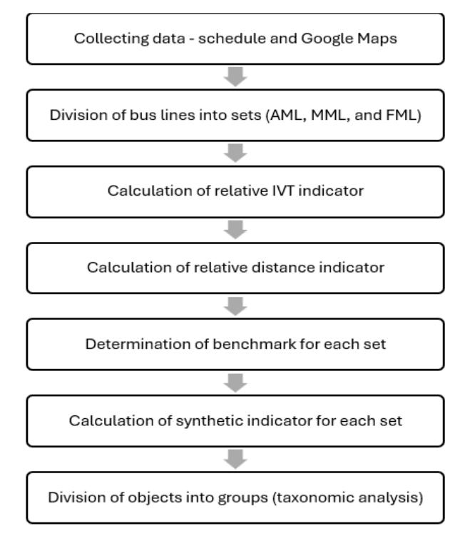
Figure 1. Research procedure.
The area selected for analysis was a special unit of local government in Poland, encompassing several cities and municipalities in the Upper Silesia and Zagłębie Dąbrowskie region. Its purpose is to foster cooperation and coordinate activities in the fields of transport, economy, spatial planning, environmental protection, and other areas significant to the region's residents. It should also be noted that this is the largest metropolitan area in Poland, with a population exceeding 2.2 million people. These characteristics make it an ideal subject for conducting research on public transport. Figure 2 presents a map of the metropolis and its location within the Silesian Voivodeship.
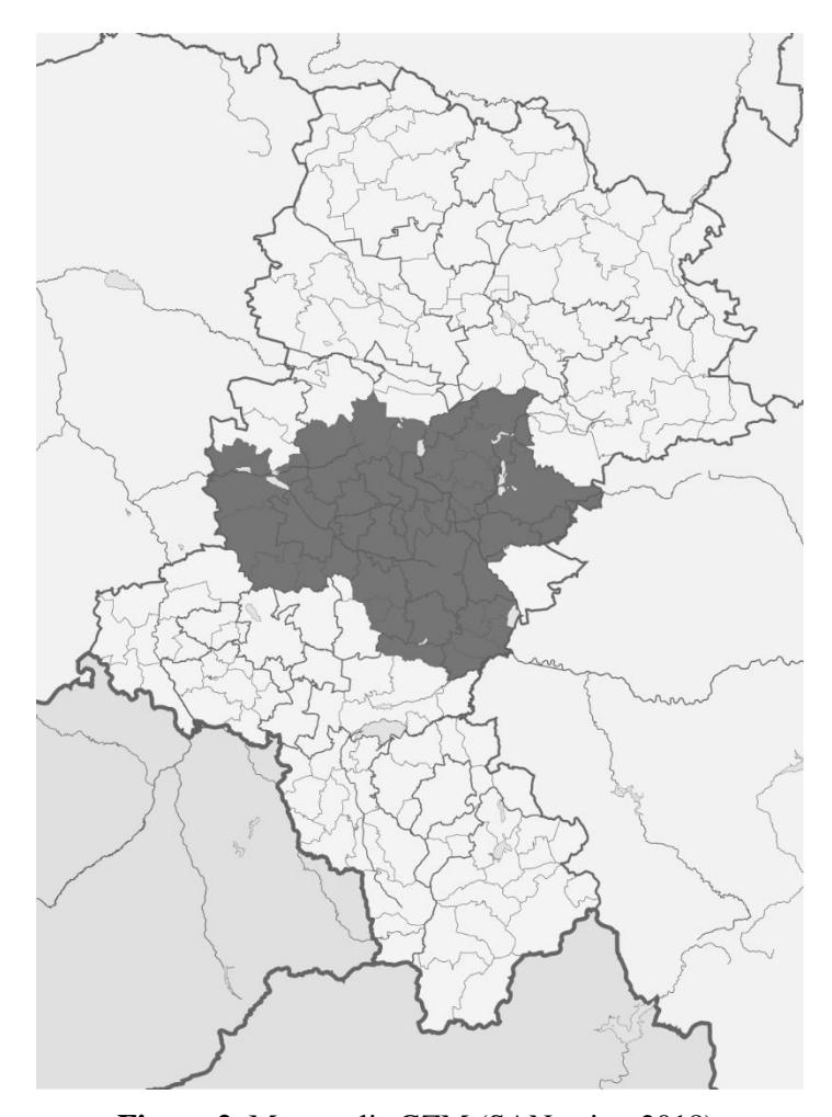
Figure 2. Metropolis GZM (SANtosito, 2018).
The analysis conducted for the purpose of this article focuses not on the specific routes of the metropolitan lines and their impact on transport accessibility but on the competitiveness of public transport in relation to private transport. However, it is worth noting that an analysis of the efficiency of metropolitan line distribution could also be an interesting research direction. Figure 3 shows the distribution of the bus lines analyzed in the article.
The data on travel time and distance for public transport came from the timetable of ZTM Katowice (ZTM, 2023), while the data for passenger cars came from Google Maps (2023). The data concern late evening hours, which allowed to avoid deviations caused by traffic congestion and random road incidents. In the case of public transport, it was the last trip of the day, while for passenger cars, it was the route determined for the average traffic volume for the same time as the public transport journey. The cross-section selected for the analysis was a working day. The analysis was conducted on three datasets (GZM, 2021b):
\[AML = \{MML \cup DML\}\]
where:
- AML = all metropolitan lines
- MML = main metropolitan lines
- FML = feeder metropolitan lines
- AP; M1, (…), M116 = metropolitan line markings
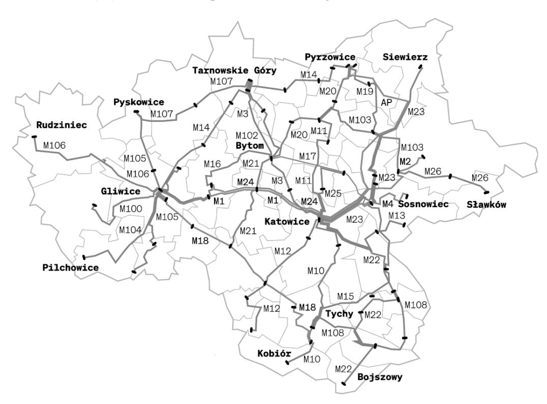
Figure 3. Metropolis lines in GZM (GZM, 2021a).
The data pertains to all metropolitan lines, so the analysis was performed for the entire population. It is also worth noting that individual metropolitan lines serve a different number of stops. Figure 4 shows the percentage of bus lines serving a given stop for the AML dataset. The number on the Y axis indicates the distance from the initial stop.
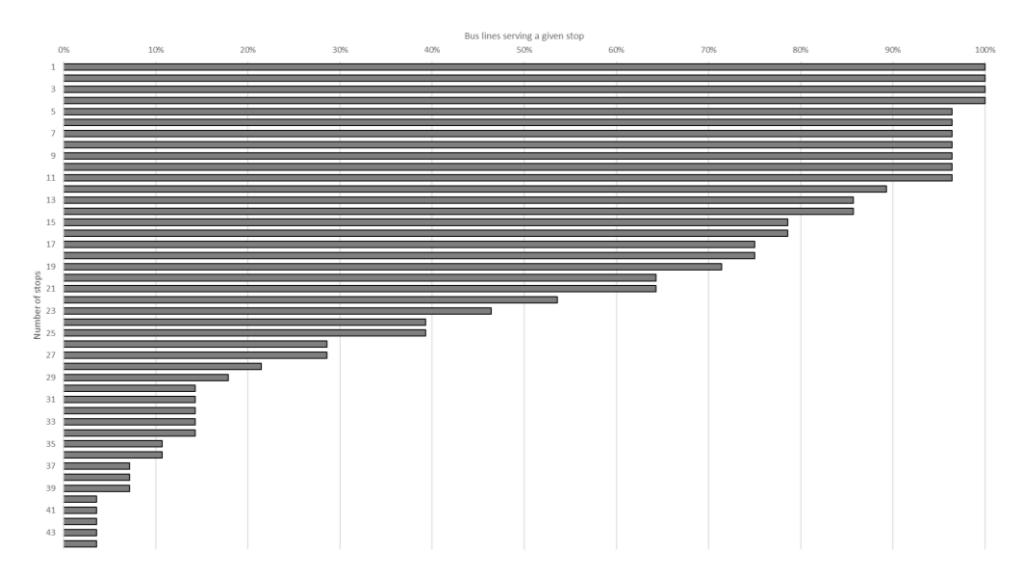
Figure 4. Percentage of bus lines serving a given stop for the AML set.
Figure 5 shows the percentage of bus lines serving each stop for the MML dataset.
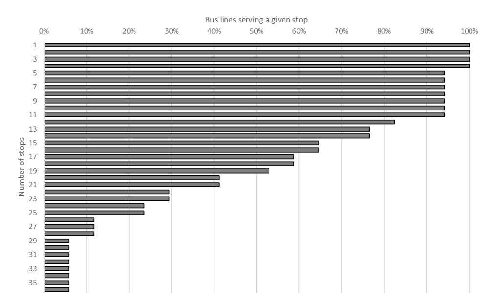
Figure 5. Percentage of bus lines serving a given stop for the MML set.
Figure 6 shows the percentage of bus lines serving each stop for the FML dataset.
Based on the obtained data, the average relative IVT indicator was calculated for each subsequent stop on the route from the initial stop:
\[rIVT_s = \frac{\left(\frac{\sum_{i=1}^{n}(T_{Bs})}{n}\right)}{\left(\frac{\sum_{i=1}^{n}(T_{Cs})}{n}\right)}\]
where:
- rIVTs = average relative IVT index for each stop along the route from the starting stop
- TBs = travel time of a bus between the starting stop and the next stop on the route
- TCs = travel time of a private car between the starting stop and the next stop on the route
- n = number of analyzed lines in a given variant
Additionally, a similar indicator was calculated for the distance traveled:
\[rD_s = \frac{\left(\frac{\sum_{i=1}^{n}(D_{Bs})}{n}\right)}{\left(\frac{\sum_{i=1}^{n}(D_{Cs})}{n}\right)}\]
where:
- rDs = average relative distance indicator for each successive stop
- DBs = distance traveled by a bus between the initial stop and each successive stop on the route
- DCs = distance traveled by a passenger car between the initial stop and each successive stop on the route
- n = number of analyzed lines in a given variant
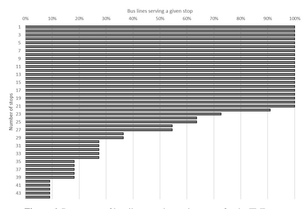
Figure 6. Percentage of bus lines serving a given stop for the FML set.
The next step of the analysis was to calculate the relative IVT indicator for each individual line:
\[rIVT_{l} = \frac{\left(\frac{\sum_{i=1}^{m}(T_{Bl})}{n}\right)}{\left(\frac{\sum_{i=1}^{m}(T_{Cl})}{n}\right)}\] where:
• rIVTl = mean relative IVT indicator for individual lines
- TBl = bus travel time between the initial stop and the next stop on the route for a given line
- TCl = car travel time between the initial stop and the next stop on the route for a given line
- m = number of stops on a given line
Based on the obtained index, a reference object was determined:
\[z0 = min\{rIVT_1\}\] where:
• z0 = reference object (taking into account the minimum value, as the rIVTl indicator is a deterrent factor).
Next, the synthetic indicator for each line was calculated for each analyzed variant:
\[S_i = \frac{rIVT_l}{z0}\] where:
• Si = synthetic indicator
The last stage of the analysis was to divide the lines into groups. The standard deviation method was used (Nowak 1990):
\[g1 \rightarrow m(s_i) - S(s_i) > S_i\] \[g2 \rightarrow m(s_i) > S_i \ge m(s_i) - S(s_i)\] \[g3 \rightarrow m(s_i) + S(s_i) > S_i \ge ms\] \[g4 \rightarrow S_i \ge m(s_i) + S(s_i)\] where:
- g1, (…), g4 = group markings
- m(si) = average value of the synthetic variable
- S(si) = standard deviation of the synthetic variable
This analysis allows for a comparison of the IVT of buses and cars for individual lines in various scenarios and its reference to the requirements presented in the line hierarchy model. Also a comparison of the distance traveled by buses and cars is presented.
Results
First, a comparison was made of the IVT parameter and travel distance for the full set of lines (AML). The analysis presents both relative and absolute values obtained (bus compared to passenger car). The averaged results for successive stops are presented in Figure 7.
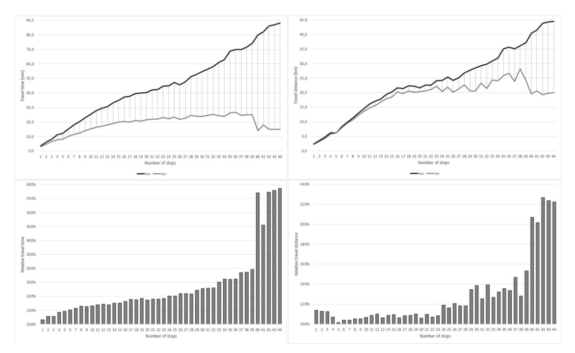
Figure 7. Bus–car IVT and distance differences for the AML set.
In the case of all metropolitan lines, public transport achieved an average IVT parameter value about twice as high (precisely 238%) as the private car. There is a relationship between the distance expressed in the number of stops and the IVT parameter: the further the journey, the less competitive the public transport was in terms of time. The point of inflection was at the 40th stop (relative IVT increase from 296% to 571%). The existence of such a point suggests calculating the average IVT for two separate ranges: for stops 1-39 (197%) and 40-44 (553%). The situation was similar for the average travel distance (again, the inflection point was visible at 40 stops): the average relative distance value for bus/car was 128%, while for the range 1-39 it was 117%, and for 40-44 it was already 219%. However, these differences were not as significant as in the case of IVT.
The above data suggest two things:
- the IVT parameter for all metropolitan lines (AML) achieved worse values than the distance parameter (which directly translates to the competitiveness of public transport),
- the existence of the inflection point at the 40th stop suggests the existence of several metropolitan lines serving the last stops (compare Figure 1), which are characterized by worse performance parameters. These will be lines from the FML group, which will be presented in a further analysis. Therefore, analysis for the main metropolitan lines group (MML) was also necessary.
The next stage of the analysis was to group the lines according to the average relative IVT indicator (benchmark). The results of the grouping are shown in Figure 8.
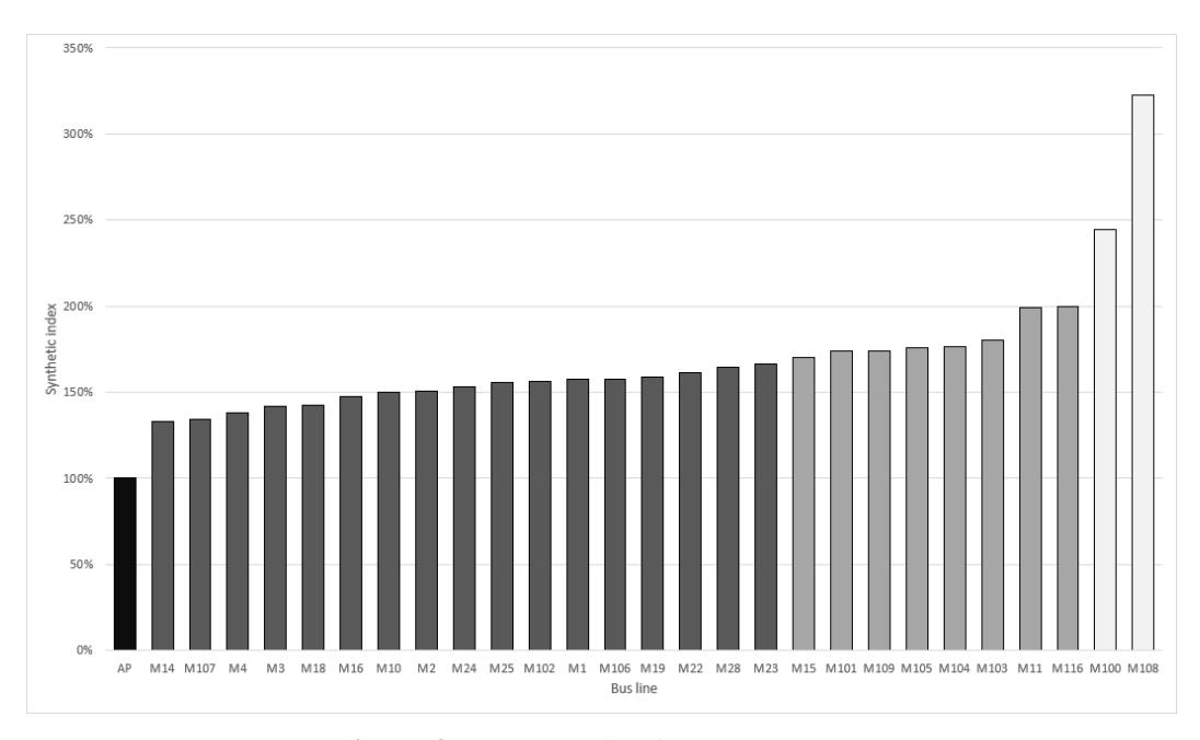
Figure 8. IVT grouping for the AML set.
The next stage of the analysis was to group the lines based on the average relative IVT benchmark. The results of the grouping are presented in Figure 8. The black color indicates very good objects (g1), dark grey – good (g2), grey – average (g3), light grey – poor (g4). Only one line (AP) was classified as 'very good', which is a line connecting Katowice with Pyrzowice Airport. Due to its destination, it is characterized by a very small number of stops and a relatively low synthetic indicator based on IVT (it is therefore a benchmark for the other lines). Most observed were 'good' lines (17 pieces). However, it should be noted that the differences between g2 and g3 were relatively small (except for two cases, i.e., M11 and M116). The worst performing lines were two feeder lines (M100, M108 – their analysis follows below). Interestingly, some feeder lines (FML) had better relative synthetic indicator values than one of the main metropolitan lines (AML), specifically M11. This situation suggests that this line should not be classified as an AML group. Nevertheless, it is described in GZM documents as amain line. The average value of the synthetic indicator for all metropolitan lines (AML) was 167%. However, it should be noted that there were at least two main breaking points: one from the M11 line and the other from the M100 line. The average value of the synthetic indicator for the AP-M103 range was 155%, while for the AP-M116 range it was 158%. These are relatively good values, which also indicate that the breaking point is the M103 line. It should also be noted that if the AP line, which has a different destination than the other analyzed lines, was removed from the analysis, the value of the synthetic indicator would be significantly lower (in this case, the benchmark would be the M14 line, and the average value of the synthetic indicator for the entire AML set without AP would be 128%, and for the M14-M103 range, it would be 118%). The analysis shows that the AML set was relatively homogeneous and in correlation with the results of relative IVT (Figure 7), it indicates a relatively high competitiveness of public transport compared to private transport. However, the IVT values were on average more than twice as bad compared to private transport.
The next step of the analysis involved comparing the IVT parameter and the travel distance for the MML set (main metropolitan lines). Once again, the analysis presents both relative and absolute values, as shown in Figure 9.
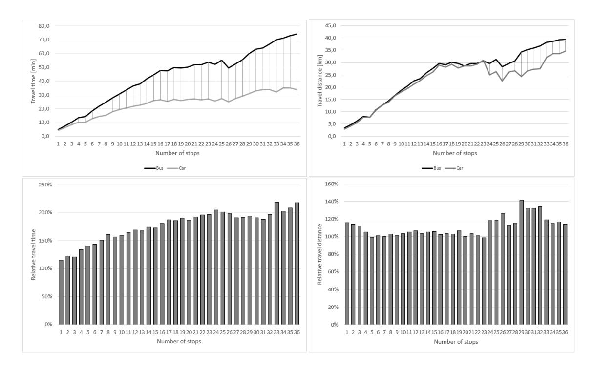
Figure 9. Bus–car IVT and distance differences for the MML set.
In the case of main metropolitan lines, public transport achieved an average IVT parameter value at the level of 177% compared to the passenger car. Again, there was a relationship between the distance expressed in the number of stops and the IVT parameter, but it was a clearly weaker relationship than in the case of the AML set. There was also no visible breakpoint. The results for the distance were also interesting, where the parameter value for the bus was only on average 111% of the value for the passenger car (thus the results were very similar to each other). The analysis indicates that the main metropolitan lines were characterized by relatively high competitiveness compared to individual transport.
The next step was to group MML lines based on the average relative IVT indicator (benchmark). The grouping results are presented in Figure 10.
The next step was to group the MML lines according to the average relative IVT benchmark. The results of the grouping are presented in Figure 10. The color codes for the different groups are the same as for the AML dataset. Again, only one line, AP, was classified as 'very good'. Seven lines were classified as 'good', eight as 'average', and one as 'poor'. As in the case of the AML dataset, the differences between g2 and g3 in the MML dataset were relatively small. The average value of the synthetic indicator for the analyzed dataset was 152%. Again, the average synthetic indicator was calculated, omitting the extreme values, i.e., the benchmark line (AP) and the weakest line (M11). In this case, the average value of the synthetic indicator was only 115%, indicating that the metropolitan lines were very similar to each other (which, compared to their relatively good IVT parameter results, again indicates their high competitiveness).
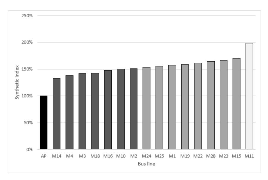
Figure 10. IVT grouping for the MML set.
The last element of the analysis was a comparison of the IVT parameter and travel distance for the FML set (feeder lines), which is presented in Figure 11.
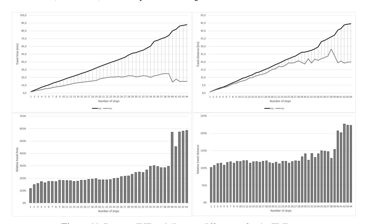
Figure 11. Bus–car IVT and distance differences for the FML set.
In the case of feeder metropolitan lines, public transport obtained an average IVT parameter value about two and a half times greater than that of the private car (exactly 248%). Interestingly, the relationship between the distance expressed in the number of stops and the IVT parameter was the weakest of all the analyzed datasets. One major breaking point was also observed, once again at the 40th stop (relative IVT increase was the same as for the AML dataset, i.e., from 296% to 571%, confirming the need for a hierarchical organization of the metropolitan lines). Once again, the average IVT was calculated for two separate intervals: for stops 1-39 (209%) and 40-44 (553%). The situation was analogous in terms of the traveled distance (although the breaking point was much weaker): the average relative distance value for bus–car was 133%, whereas for intervals 1-39 it was 123%, and for 40-44 it was already 216%.
The last stage of the analysis was to group the lines according to the average relative IVT indicator (benchmark). The results of the grouping are presented in Figure 12.
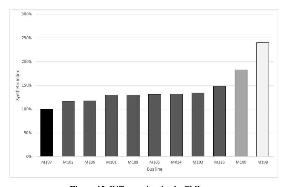
Figure 12. IVT grouping for the FML set.
The final stage of the analysis involved grouping the lines according to the average relative IVT indicator (benchmark). The grouping results are presented in Figure 12. The color designations for each group are the same as for the AML and MML datasets. Once again, only one line (M107) was classified as 'very good', while 8 were classified as 'good', 1 as 'average', and 1 as 'poor'. In the analyzed dataset, the differences between groups 1 and 2 were relatively small. The average value of the synthetic indicator for the analyzed FML dataset was 142%. We decided to calculate the average synthetic indicator excluding the outlier values, i.e., the average line (M100) and the poor line (M108). In this case, the average value of the synthetic indicator was only 127%, indicating high homogeneity of the FML dataset. However, the difference between the synthetic indicator values for the entire FML dataset and for the dataset with the outlier observations removed was not as significant as it was for the MML dataset.
The conducted analysis indicates that the public collective transport carried out on the metropolitan lines of the Metropolis GZM as characterized by a relatively good IVT parameter and relative distance. The best results were achieved by the main metropolitan lines, while the feeder lines performed worse. Such a situation is entirely understandable and consistent with the strategy adopted by the ZTM in Katowice. Table 2 presents the summary data for all analyzed variants.
However, it should be noted that metropolitan public transport lines (both main and feeder) primarily connect major points in the city, which means that they are rarely used as the sole means of transport. In the case of needing to get to other parts of the city outside of the city center or to smaller towns/villages, the IVT parameter will likely increase drastically. Additionally, there may be a need to wait for the next ride. Furthermore, during peak hours, the number of passengers is significantly higher, which can lead to overcrowding on buses (Pan, Waygood and Patterson, 2022).
| AML [%] | MML [%] | FML [%] | ||
|---|---|---|---|---|
| All lines | Average relative IVT | 237,6 | 177,0 | 247,9 |
| Average relative distance | 128,4 | 111,0 | 133,4 | |
| Average relative distance | 167,4 | 152,4 | 141,9 | |
| Standard deviation of Si values | 39,3 | 19,6 | 36,9 | |
| Lines without outliers | Average relative IVT | 197,2 | - | 208,7 |
| Average relative distance | 117,1 | - | 122,8 | |
| Average relative distance | 127,6 | 114,8 | 126,5 | |
| Standard deviation of Si values | 28,4 | 7,9 | 12,9 |
Table 2. Summary data for AML, MML, and FML datasets
Discussion
Travel time is a fundamental measure in many accessibility studies, evaluating how easily individuals can reach various destinations for different activities within a specific travel time limit using a particular mode of transport (Hansem, 1959; Farber and Fu, 2017). Comparison of the IVT parameter of public transport lines in relation to private cars is of great importance for urban planning, particularly for the transport policy of a given area. This comparison allows for a direct assessment of the efficiency of public transport journeys. In transport policies, many cities and scientific articles place emphasis on parameters such as stop network density (Pandey, Lehe and Monzer, 2021), accessibility for people with disabilities (Odame et al., 2023; Muñoz, 2021), type of transport tariff (Świrek et al., 2023), ticket prices, travel comfort, and safety (Tomas and Rahman, 2022). Also, the growth of public transport ridership is limited by several factors, including fixed schedules and routes, low population density, and travelers' attitudes (Alam, Hilary and Qiong, 2015). From the passenger's perspective, the time spent on the journey is extremely important (often even the most important). A key factor in the growth of public transport ridership is the decrease in users' perceived marginal costs, which includes travel time (Beirão and Cabral, 2007; De Vos et al., 2016; Litman, 2017). It should also be emphasized that travel time is considered one of the main factors characterizing the quality of public transport. (Xin, Fu and Saccomanno, 2005; Eriksson, Friman and Gärling, 2008). In the case where public transport achieves high IVT values compared to alternatives, the potential passenger is likely to choose an alternative mode of transport. Existing scientific publications clearly indicate that the topic addressed in the article is both relevant and necessary in the debate at both the academic and practical levels.
The above situation makes it natural to consider incorporating the IVT parameter in the planning of a city's transport policy. Public transport lines serving as the main metropolitan connections should have an IVT parameter as close as possible to that of private cars. However, it is obvious that as the distance increases, the IVT parameter for public transport will become worse compared to private transport. This is directly related to the conflict between two basic transport principles, namely directness of travel and travel time. Direct public transport will always have a higher IVT parameter. This situation will be even more visible for the remaining lines that serve local connections. It is necessary to find a balance between the costs incurred (number of serviced lines, their routes, available fleet, frequency, etc.) and the IVT parameter. A potential solution to this problem may be to base the design of the transport network on a simulation approach. In that case it is important to accommodate the stochastic realities of traveler behavior in a transit network design solution (Nnene, Joubert and Zuidgeest, 2023).
A good practice when creating transport policy for a city/region would be to consider the IVT parameter and analyze potential ways to improve it. Such an approach would allow for a much broader approach to the issue of public transport efficiency and could contribute to improving its quality.
It should also be noted that an increasing number of publications seem to highlight the importance of disparities between public transport and private cars (Renne, 2016; Moya-Gómez and Geurs, 2018). These conclusions correspond very well with the results obtained in the research conducted for this article. However, many accessibility studies usually estimate travel times for cars and public transport for hypothetical destinations or are confined to locations with specific functions, such as workplaces or hospitals (Durán-Hormazábal and Tirachini, 2016; Stępniak et al., 2019). These results cannot be compared with those from the present article, as they do not include the location of the stops themselves but rather the placement of traffic generators. However, both approaches seem to complement each other, as the speed of public transport does not necessarily align with the efficient distribution of stops, and vice versa. Spatial approaches are also becoming more common, utilizing tools such as GIS software (Calegari, Celino, and Peroni, 2016), GPS data (Luo et al., 2017), or city cards (Pelletier, Trépanier, and Morency, 2011). Similarly to the main destination points, these studies cannot be directly compared when it comes to the geographical approach. Once again, one approach will complement the other, rather than serve as a research alternative.
It also should be noted that relatively few publications addressed the differences in travel times between public transport and private cars (Liao et al., 2020). In this study, the researchers compared travel times by private car and public transport in four cities (São Paulo, Brazil; Stockholm, Sweden; Sydney, Australia; and Amsterdam, the Netherlands). The results suggest that using public transport takes on average 1.4 to 2.6 times longer than driving a car. These findings are very consistent with the results of the research conducted for this paper. In the Metropolis GZM, public transport travel takes on average 1.77 times longer for major public transport routes and up to 2.48 times longer for other routes. These results indicate that Metropolis GZM is very similar in terms of public transport time efficiency to São Paulo, Stockholm, Sydney, and Amsterdam. It is important to continue emphasizing the fact that there is still a lack of sufficient studies directly comparing travel times between private cars and public transport, which represents a significant research gap. Therefore, determining the travel time between individual stops (by private car and public bus) appears to be a necessary task.
However, it should be noted that the conducted study is not without limitations. A potential limitation that may have affected the results of the study is the choice of time period (workdays, last trip). It may turn out that the results for other periods (e.g. Saturdays, Sundays, and holidays) will be different. Similarly, in the case of choosing a different time, the IVT during peak hours will certainly be much higher. However, the question arises as to whether the relative IVT compared to a private car will increase, decrease, or remain unchanged. However, choosing night-time hours seems to be a logical choice, as it maximizes the reduction of external factors (traffic congestion, accidents, and collisions).
Future research could focus on determining the IVT parameter for all lines in the Metropolis GZM compared to private vehicles. Such an analysis would allow for the overall assessment of the urban transport system in the Metropolis GZM and its competitiveness compared to private transport. Another avenue for research is to determine differences in time accessibility across other large cities and compare the results obtained. An interesting research direction is also the application of spatial approaches to visualize the results. Additionally, econometric models (e.g., spatial regression) could be used to identify correlations between demographic factors
(e.g., population density, income, etc.) and the IVT indicator results for specific areas. Finally, incorporating qualitative factors into the analysis could also provide valuable insight and be an intriguing direction for future research.
Conclusions
In-vehicle time disparity of major metropolitan lines and private car was observed in Metropolis GZM. This situation can significantly affect the competitiveness of public transport compared to private transport. Also, the IVT parameter is extremely important from the perspective of urban planning. It is worth noting that the analysis concerned only the core of the metropolitan transport, i.e., the metropolitan lines. In the case of analyzing the entire system, the relative value of the IVT parameter for bus–car would be significantly higher.
The issues raised in this paper are relevant to every active and potential user of public transport, making it of interest to city dwellers and those interested in the efficiency and competitiveness of public transport. Despite the significant importance of the IVT parameter for the efficiency of urban public transport and city planning, there are not many publications in the subject literature that specify the value of this parameter in relation to alternative modes of transport (particularly private cars). This is a relatively strange phenomenon, especially taking into account many actions in the field of reducing private car dependence.
This article may therefore be a stimulus for academic debate on this topic and guide future research directions. The article should be of interest to researchers working on public transport. However, it is worth noting that urban transport is an integral part of urban planning, so the thematic scope of the article should also be relevant to planners from other fields.