
INTRODUCTION
Krukut River is one of rivers in Depok that is included in the Krukut watershed. Krukut River has \(\pm\) 48 km in length upstream from Situ Citayam Bogor and merges at Ciliwung River which enter into Jakarta Bay. Originally the Krukut River was a clean river and became a tourist destination under the Dutch government. Population growth and surrounding activities put pressure on the Krukut River conditions. In recent years, the Krukut River has become clogged with rubbish so that during the rainy season it causes flooding.
The disposal of various types of waste and rubbish containing various types of pollutants, both biodegradable and non-biodegradable will cause more and more of the pollutant load received by the river. Activities around the Krukut River are settlements. This type of pollutant source will potentially pollute times. According to the Depok Spatial and Regional Plan 2012/2032, the Krukut River's fluctuations are very dependent on rainfall in the catchment area. High flow occurs during the rainy season and decreases during the dry season. Normal discharge of Krukut River is> 70 m 3 /second. Land use in the Krukut watershed is divided into 12 land use classes, namely primary, secondary forest, mixed gardens, plantations, settlements, swamps, rice fields, shrubs/ponds, ponds, open land, fields / fields, and water bodies.
Rivers that receive pollutants are able to recover quickly (selfpurification), especially against wastes that cause a decrease in oxygen levels (oxygen demanding wastes) and waste heat. The ability of a river to recover from pollution depends on the size of the river and the rate of river water flow and the volume and frequency of incoming waste. The ability of a river to recover itself from pollution is influenced by (1) the flow rate of river water, (2) related to the type of pollutants that enter the body of water. Nonbiodegradable compounds that can damage life in the riverbed, cause massive fish death, or occur biological magnification in the food chain (Miller, 1975).
In principle, the river has the ability to recover from pollution. Factors that influence the ability to recover river waters are the structure of the waters, elevation, current speed, exposure to sunlight and the amount of dissolved oxygen in the water. Organic pollutants that enter will be degraded by microorganisms into compounds that can be utilized by phytoplankton and other river animals, deposited or carried by the flow of water. The ability to recover river waters can be calculated using the Streeter-Phelps method.
The Streeter-Phelps Mathematical Method is a method based on a mathematical model developed by Streeter and Phelps. This study is about the automatic purification process of water bodies. Steeter Phelps' findings show that when pollution enters a body of water that originally had a DO saturated level, the Ds of dissolved oxygen content from the river immediately thawed with an initial deficit, Do. Curve A represents a scenario where the polluted river recovers without passing anaerobically (DO = 0). Curve B presents a case where pollution causes a river to become anaerobic septic (Lin and Lee, 2007).
Mathematical models have been developed for river water purification. Because river ecology is very dependent on the amount of dissolved oxygen in the water, this dissolved oxygen (DO) seems to be an easy criteria to use to measure the level of river pollution as far as organic pollution is concerned. However, even the term organic pollution includes a large number of different materials and questions that assess the burden of this pollutant are increasing. Taking into account that the effect of all types of organic matter will be dissolved oxygen consumption, it usually measures the burden of organic pollution with the amount of oxygen needed to actually oxidize this charge by bacteriological damage, ie by biological oxygen demand (BOD). Current analysis is related to polluted water in rivers. The validity of the prospecting use of the Model depends very much on the validity of the equation that has been used and this depends on the knowledge of accurate, diffusion and reaeration hydraulic parameter advections. This parameter is quite well known as a theoretical approach when compared with biodegradation and other phenomena. Under these conditions, a complete understanding of the mechanism of self-purification can be obtained. This mathematical model is very helpful for studying oxygen in rivers. This model is only limited to two phenomena, namely:
- 1. The process of reducing dissolved oxygen (deoxygenation) due to bacterial activity
- 2. The process of increasing dissolved oxygen (reaeration) caused by turbulence that occurs in river flow.
River automatic purification capacity that has been limited by the relatively low DO saturation level is threatened by waste discharged into it at varying intervals. Some non-biodegradable and acidic wastes have also been found to interfere with the river's automatic purification process (Omole, 2016).
RESEARCH METHOD
This research was conducted in Krukut River Depok along ± 9.04 km. The study sites were divided into 7 sampling points located in Beji District, Pancoran Mas District, and Limo District. The location of 7 sampling points is shown in Table 1 and Figure 1. Pollutant sources are determined from the results of surveys directly in the field so that pollutant sources obtained consist of pollutant sources and non-source sources.
The hydraulics and morphology characteristics of the river that have been obtained from observations and measurements, tabulated and analyzed descriptively. River characteristics measured geometrically consist of flow, flow velocity, slope, and depth of the river.
River Discharge (m3 /sec) = Current velocity (m/s) x river cross-sectional area (1)
Current Speed = Distance/time (m/s) (2)
Slope (d/d) = d right / d left (3)
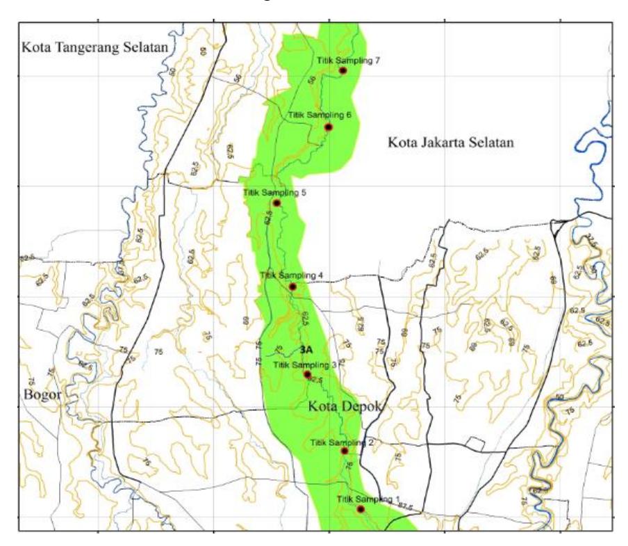
Figure 1. Sampling point at Krukut River
Table 1. Sampling point at Krukut River Depok, West Java
| Sampling | Titik Koordinat | Distance each point | |
|---|---|---|---|
| point | E | S | (km) |
| 1. | 106° 48' 20,080" | 6° 23' 57,000" | 0 |
| 2. | 106° 48' 10,520" | 6° 23' 57,720" | 1,15 |
| 3. | 106° 48' 50,760" | 6° 22' 56,280" | 1,24 |
| 3A | 106° 48' 48,760" | 6° 22' 40,280" | |
| 4. | 106° 47' 40,400" | 6° 21' 54,760" | 1,45 |
| 5. | 106° 47' 30,760" | 6° 20' 10,680" | 1,9 |
| 6. | 106° 48' 0,360" | 6° 20' 24,720" | 2,16 |
| 7. | 106° 48' 10,880" | 6° 19' 51,000" | 1,14 |
| TOTAL | 9,04 |
14 Jurnal Teknik Lingkungan Vol.26 No. 2 Yuni Sesempuli, Bambang Iswanto, dan Diana Irvindiaty Hendrawan.
Information :
1-7 is the main sampling point.
3A is a sampling point in Creek of Krukut River .
Streeter Phelps is used to determine the ability of rivers to degrade pollutants. In this case there are two phenomena, namely the process of reducing dissolved oxygen (deoxygenation) due to bacterial activity in degrading organic matter present in water and the process of increasing dissolved oxygen (reaeration) caused by turbulence that occurs in stream currents. Streeter - Phelps Oxygen Reduction (deoxygenation) process states that the rate of biochemical oxidation of organic compounds is determined by the concentration of residual organic compounds.
dL/dt = K'.L (4)
with
L : concentration of organic compounds (mg/L)
t : time (day)
K : first order reaction constants (day-1)
If the initial concentration of an organic compound as BOD is Lo which is stated as ultimate BOD and Lt is BOD at time t, then the above equation is stated as: dL / dt = - K'.L
The results of the integration of the above equation during the deoxygenation period are:
Lt = Lo.e (K'.t) (5)
Determination of K 'can be done by:
- 1. Logarithmic difference method,
- 2. Moment method (Moore et al method), and
- 3. Thomas method.
The deoxygenation rate due to organic compounds can be expressed by the following equation:
rD = -K'L, with K ': first order reaction rate constants, day -1
L : BOD ultimate at the requested point, mg/L
If L is replaced by Loe-K't, equation becomes
\[rD = -K'Loe^{-K'.t},\] with:
Lo: BOD ultimat at the discharge point (after mixing), mg/L. The process of increasing dissolved oxygen (reaeration). The oxygen content in the water will receive additional effects due to turbulence so that the oxygen transfer takes place from the air to the water and this process is a reaeration process. This oxygen transition is expressed by the reaeration rate equation:
\[rR = K^2 (Cs - C)\] with
K`2 : reaeration constant, day-1 (natural number base)
Cs : saturated dissolved oxygen concentration, mg/L
C : dissolved oxygen concentration, mg/L
The reaeration constant can be estimated by determining the current characteristics and using one of the empirical equations. The O'Conner and Dobbins equation is a common equation used to calculate reaeration constants (K'2).
\[K'2 = 294 (DL.U)^{1/2} H^{3/2} (6)\] with
DL : Molecular diffusion coefficient for oxygen, m2 /day
U : Average current speed, m/sec
H : Average current depth, m
The variation in the coefficient of molecular diffusion with temperature can be determined by the equation:
DLT = \[1,760 \times 10^{-4} \text{ m}^2/\text{d} \times 1,037 \text{ T}^{-20}\] (7)
with
DLT : Oxygen molecular diffusion coefficient at temperature T, m2 /day
1,760 x 10-4 : Oxygen molecular diffusion coefficient at 20 oC
T : temperature, oC
The value of K`2 has been estimated by the Engineering Board of Review for the Sanitary District of Chicago for various water bodies
16 Jurnal Teknik Lingkungan Vol.26 No. 2 Yuni Sesempuli, Bambang Iswanto, dan Diana Irvindiaty Hendrawan.
Table 2 Reaeration Constants K2
| Water body | (base e) a |
|---|---|
| Small ponds and backwaters | 0.10-0.23 |
| Sluggish streams and lage lake | 0.23-0.35 |
| Large streams of low velocity | 0.35-0.46 |
| Large sreams of normal velocity | 0.46-0.69 |
| Swift streams | 0.69-1.15 |
| Rapid and waterfalls | >1.15 |
Oxygen sag curve
If it is assumed that the times and waste are completely mixed at the point of discharge, then the concentration of the constituents in the waste water mixture at x = 0 is
\[Co = \frac{Qr Cr + Qw Cw}{Qr + Qw} \tag{7}\] with:
Co = Initial constituent concentration at the point of discharge after mixing, mg/L
Qr = Flow rate times, m 3 /sec
Cr = Concentration of constituents in the times before mixing, mg/L
Cw = Concentration of constituents in wastewater, mg/L
As a description of the simulation of the streeter phelps method the following formulas can be found:
V (m / day) = to find t in days, used to find the BOD value on a particular day.
Formula : V (m/sec) x 86400
T in days is used in the BOD formula
\[L = Lo e^{-kt} (8)\] where :
Lo = Ultimate BOD at the point of mixing
L = BOD at time t (in days)
V = BOD decay constant (BOD decay)
t = Time
Q manning (m3 /sec)
\[\frac{1}{n}AR^{2/3}S^{1/2} \tag{9}\]
Q = discharge (m3 /sec)
V* = velocity (m/sec) V* =√g HS
\[K = \frac{E}{H \times V} \tag{10}\]
K = Dispersion constant (m2 /sec)
H = depth (m)
V * = average speed (m /sec)
E Lat = Lateral coefficient (m2 /sec)
\[E Lat = 0.6 H V^*\] (11)
H = average depth (m)
Lateral Mixing Length (Lm)
\[Lm = 0.4 V \frac{B^2}{E Lat}\] (12)
Lm = mixing distance (m)
H = Depth (m)
V = Velocity
B = Width (m)
Vs = deposition speed of BOD dispersion
The formula for calculating the pollution load deposition coefficient is:
Depositional constant at times (d-1) or settling rate (k3)
\[Ks = Vs/H \tag{13}\]
The formula for calculating the reaeration coefficient is:
\[Ka = 3.9 \frac{V^{0.5}}{H^{1.5}} \tag{14}\]
18 Jurnal Teknik Lingkungan Vol.26 No. 2 Yuni Sesempuli, Bambang Iswanto, dan Diana Irvindiaty Hendrawan.
\[krT = ksT + kdT\] (15)
Kd = \[(0.376 \times BOD (mg/L)/87.12\] (16)
The formula for calculating the pollutant load decay coefficient is kd = -b
\[kd = na + b \sum y - \sum y' = 0\]\[a \sum y + b \sum y^2 - \sum yy' = 0\]
By substituting the two equations above it can be seen the values of a and b.
Where :
n = Amount of data processed a = -bL
b = -k (base e)
L = -a/b
Y = yt, mg/L
Y' = (yn+1 – yn-1)/2 ∆t
BOD Enter = Lo : e-kt where:
\[LO = (LO2 + LO3) e -kd\]
Q Enter = Q in between point 2 and 3
\[\frac{BOD2 - BOD3}{BOD2 - BODin} \tag{17}\]
Where :
= Correction of the BOD Decay coefficient = 1.047
= Correction of the BOD Settling coefficient = 1.024
= Correction coefficient DO remain = 1,024
SOD = Correction of SOD coefficient uptake = 1.06
Ka = Constant reaeration
K SOD = SOD constant value of the uptake is assumed to be 1
K (T) = - K20 T-20C
T = Temperature
BOD Streeter Phelps
\[L = Lo.e^{-kt}\]
\[L_{1-2} = BOD V1 \cdot e -kd_{1-2} \cdot t_{1-2}\]
\[L_{2-3} = BOD V1-2 \cdot e -kd_{2-3} \cdot t_{2-3}\]
BODin
\[BODin = \frac{Q1 - 2xBOD2 + Q2 - 3xBOD}{Q1 - 2 + Q2 - 3}\] (18)
Cs = DO Saturation
\[\ln osf = -139,3441 = \frac{1,575701 \times 10^5}{T\alpha} - \frac{6,642308 \times 10^7}{T\alpha^2}\] (19)
DO Streeter Phelps
Ka = rearation rate (/ day)
\[C = Cs - \left\{ \frac{kd}{ka} - kt \left[ e \left( -kr \frac{x}{v} \right) - e(-ka \frac{x}{a}) \right] \right\} Lo - (cs - co)e \left( -ka \frac{x}{a} \right)\] (20)
Kd = decay rate (/ day)
Lo = initial BOD concentration (mg/L)
Cs = DO value saturation or saturated oxygen level (mg/L)
C = DO concentration (mg/L)
RESULT AND DISCUSSION
The calculation using the Streeter Phelps method is performed to determine the degradation rate of the Krukut River. Therefore, it must be known in advance the factors that influence Krukut River. Krukut River is a domestic area with a variety of trading businesses and schools. These various types of business produce various types of waste that will affect the degradation process and the rate of deposition speed in the Krukut River. Not infrequently during the rainy season it is not uncommon for floods to occur. In addition, the types of waste that enter can affect the rate of degradation. Streeter Phelps calculation is used to find out the Kd, Ks, and Ka. Where Kd means the degradation constant (decomposition) serves to show the magnitude of the rate of decomposition of organic matter by aerobic microorganisms in water. Ks means settling
constant (d-1) to find out the settling speed at Kali. And Ka means the reaeration constant serves to show the rate of absorption of atmospheric oxygen into the waters.
Land use change is the rate of land used which will ultimately have an impact on water conditions. Relamation of wetlands into built up areas is due to urbanization and accelerated development in watersheds. This will change the landscape and affect the aquatic ecosystem (Guang et al, 2016).
An increase in population due to urbanization will cause pressure on rivers. The natural ability of rivers to selfpurification is reduced because the pollutants that enter are greater than the ability of self-purification. The ability of river self-purification is influenced by the physico-chemical conditions in the river in addition to the basic characteristics of the river (Prasad et al, 2016).
The physical characteristics of the waters are influenced by the discharge, the basic type of waters and the topography. While the temperature affects the solubility of oxygen in water and affects the processes that occur in the waters. Oxygenated waters are identified as healthy waters and have good self-purification abilities. Oxygen content in waters is affected by turbulence of flow. Pollutants that enter the river will inhibit the flow of water and reduce turbulence. As a result, the oxygen content will decrease and to be influence to biotic factors (Eliman et al, 2015).
River bed sediments play a role in biogeochemical processes and as an ecological response to pollution. Microorganisms in sediments play an important role in the nutrient cycle and degradation of organic matter. The presence of toxic pollutants and heavy metals can destroy microorganisms in the sediments so that degradation is not going well (Li et al, 2016).
The ability of self-purification in rivers is affected by dissolved oxygen content. High organic pollution will increase the value of BOD in water, consequently DO values will be low. Usually DO content will be low in the river downstream. Besides being caused by contamination that is increasingly high is also influenced by the lower current speed. To reduce stress on the river, pollutants must go through wastewater treatment (Satya and Narayan, 2018).
BOD concentrations in the Krukut River ranged from 4.41 to 91.25 mg/L with a quality standard of 2 mg/L. DO concentrations ranged from 4.45 to 6.31 mg/L with a quality standard of 3 mg/L. COD concentrations ranged from 16.56-124.8 mg/L with a quality standard of 10 mg/L.
Krukut River current velocity is influenced by elevation. Krukut River elevation is in the range of 80 meters above sea level to 56 meters above sea level, with the measurement results of the current speed of 0.286-1.29 m/sec. High current velocity and fluctuation in current causes dissolved oxygen (DO) to be high. Means that value can decipher contamination. High DO concentrations play a role in increasing the work of microorganisms in degrading pollutants. High aeration helps the growth of microorganisms. Microorganisms will degrade organic matter into dissolved solid particles and suspended particles. BOD concentrations in Krukut River ranging from 20-80 mg/L exceed the quality standard set at 2 mg/L.
The difference of BOD values in field with significant Streeter Phelps modeling calculations shows that naturally polluting concentration values can be suppressed in the range of 20-80 mg/L which can only be accepted by times. This will be related to the rate of degradation of oxygen absorption and the rate of degradation of decomposition (Kd) showing the ability of microorganisms to oxidize organically. Under certain conditions, the Kd value of waters can be greater because of the deposition factors and sediment effects. Therefore, constants in the field need to consider other constants that can increase the Kd value, namely the addition of constants from the particle deposition process (Ks), so that the constant value changes to Kr = Kd + Ks.
The rate of increase in dissolved oxygen (Ka) with a value range of 1.586-4.542 d-1 Ka. The default value of Ka is 1.494 d-1 which exceeds the standard value indicating that the Krukut River aeration is quite good. If the DO concentration is seen in the range of 4.45–6.3 mg / L it means that the concentration of dissolved oxygen is slightly, so the BOD concentration is quite high. With the rate of absorption of oxygen (Ka) which is large enough means that the influence of the speed of the current that causes water turbulence is quite good times. Also seen in Figure 4.1. Krukut Kali Discharge which continues to increase in May with a peak peak of 7.889 m3 / sec indicates that the heavier the water discharge the better the rate of degradation. The decomposition degradation rate (Kd) indicates the ability of microorganisms to oxidize organically. The results obtained range values of 0.285-0.374 d-1 standard Kd value of 0.501 d-1 means that the Kd in Krukut River is small meaning the range is less than the standard value. This means that the process of decomposition of organic matter by microorganisms is slow. For the sedimentation rate (Ks) the range of 0.070-0.096 d-1 with a standard value should be 0.751 d-1 which means that the Krukut River deposition process is quite slow. From table 3-5 it can be seen that using the Streeter Phelps model, the ability of the Krukut River to accept BOD pollutants is 10.34-84.05 mg / L.
The natural purification process depends on the absorption and renewal of oxygen from the surface of the water. The presence of oxygen is very important for bacterial growth to degrade pollutants biologically and chemically. The ability of natural river purification depends on natural factors such as currents, depth, discharge and temperature. Turbulence in rivers helps rivers become cleaner while slow flows tend to have septic conditions due to low oxygen content (Karthiga et al, 2017).
The river has the ability to purify naturally and its ability to reflect the level of health of the river. Pollution control that enters and maintains river flow patterns is an effort to control the river's purification capabilities. Bacteria at the bottom of the waters play a role in degrading pollutants but in general rivers have a low purification ability if polluted by heavy metals (Tian et al, 2011).
Mathematical models can be applied to describe the level of effort to maintain river sustainability. The model also illustrates the effect of oxygen on water. Incoming pollutants can be described at a level acceptable to rivers (Pimpunchat et al, 2009). The simulation using the Streeter-Phelps model to see the water quality is very sensitive using BOD and NH3-N parameters. The Streeter-Phelps model can also be used with limited data (Fan et al, 2012).
Table 3. Calculation of Streeter Phelps In March 2017 in Krukut River
| Sampling point | |||||||||||
|---|---|---|---|---|---|---|---|---|---|---|---|
| Observation | 1 | 2 | 3 | 4 | 5 | 6 | 7 | Information | |||
| Suhu (°C) | 29.40 | 29.30 | 29.25 | 30.20 | 29.30 | 28.70 | 28.60 | ||||
| v (m/sec) | 0.300 | 0.570 | 0.700 | 0.815 | 0.839 | 0.990 | 1.290 | Current speed | |||
| v (m/dayi) | 25920 | 49248 | 60480 | 70416 | 72490 | 85536 | 111456 | Current speed | |||
| x (m) | 0 | 1150 | 2390 | 3840 | 5740 | 7900 | 9040 | Cumulative distance | |||
| t (day) | 0.001 | 0.02 | 0.04 | 0.05 | 0.08 | 0.09 | 0.08 | Time | |||
| H (m) | 1.300 | 1.233 | 1.900 | 1.550 | 1.590 | 1.220 | 1.130 | River depth | |||
| Sampling j | point | |||||||
|---|---|---|---|---|---|---|---|---|
| Observation | 1 | 2 | 3 | 4 | 5 | 6 | 7 | Information |
| B (m) | 8.33 | 6.43 | 3.71 | 5.39 | 5.49 | 6.42 | 5.37 | Wide |
| D (m/m) | 0.854 | 1.031 | 0.888 | 2.044 | 1.117 | 0.827 | 1.106 | River slope |
| Elevation (m) | 80 | 75 | 62.5 | 62.5 | 62.5 | 62.5 | 56 | Elevation |
| S (m/m) | 0.5477 | 6.2539 | 8.6309 | 10.7366 | 12.2904 | 14.6931 | 17.4644 | Slope |
| Q (m³/sec) | 3.249 | 4.519 | 4.934 | 6.809 | 7.324 | 7.754 | 7.828 | Discharge |
| Q (m³/sec) Manning | 18.653 | 40.385 | 45.891 | 47.426 | 65.833 | 65.470 | 46.773 | Manning Discharge |
| R (m) | 1.0719 | 0.8776 | 0.9958 | 0.6883 | 0.9525 | 0.9722 | 0.7562 | Wet cross section |
| A (m²) | 10.83 | 7.93 | 7.05 | 8.36 | 8.73 | 7.83 | 6.07 | Cross- sectional area |
| N | 0.45 | 0.45 | 0.45 | 0.45 | 0.45 | 0.45 | 0.45 | Roughness coefficient |
| U* (m/sec) | 2.643 | 8.697 | 12.683 | 12.777 | 13.846 | 13.261 | 13.914 | Shear velocity |
| E (m²/sec) | 0.020 | 0.014 | 0.003 | 0.011 | 0.011 | 0.027 | 0.034 | Dispersion |
| E lat (m²/sec) | 2.062 | 6.434 | 14.459 | 11.883 | 13.209 | 9.707 | 9.434 | Lateral dispersiona |
| Lm | 0.098 | 0.054 | 0.070 | 0.066 | 0.064 | 0.061 | 0.070 | Miing distance |
| K | 0.001 | 0.001 | 0.001 | 0.001 | 0.001 | 0.001 | 0.001 | Dispersion constant |
| vs (m/sec) | 0.1 | 0.1 | 0.1 | 0.1 | 0.1 | 0.1 | 0.1 | Sedimantation speed |
| BOD (mg/L) | 84.05 | 43.24 | 28.82 | 32.43 | 25.22 | 49.23 | 91.25 | BOD field |
| BOD in (mg/L) | 72.06 | BOD minxture | ||||||
| q in (m³/dtk) | 1.51 | QC (mixed discharge) | ||||||
| DO (mg/L) | 6.10 | 5.43 | 6.31 | 4.45 | 5.43 | 5.54 | 5.56 | |
| θkd | 1.047 | 1.047 | 1.047 | 1.047 | 1.047 | 1.047 | 1.047 | Decomposition coefficient correction factor |
| θks | 1.024 | 1.024 | 1.024 | 1.024 | 1.024 | 1.024 | 1.024 | Settling coefficient correction factor |
| θka | 1.024 | 1.024 | 1.024 | 1.024 | 1.024 | 1.024 | 1.024 | Aeration coefficient correction factor |
| Sampling point | ||||||||
|---|---|---|---|---|---|---|---|---|
| Observation | 1 | 2 | 3 | 4 | 5 | 6 | 7 | Information |
| θ SOD | 1.06 | 1.06 | 1.06 | 1.06 | 1.06 | 1.06 | 1.06 | Correction factor |
| coefficient up take | ||||||||
| Kd | 0.363 | 0.187 | 0.124 | 0.140 | 0.109 | 0.212 | 0.394 | Decomposition constant |
| Ks | 0.077 | 0.081 | 0.053 | 0.065 | 0.063 | 0.082 | 0.088 | Settling constant |
| Ka | 1.452 | 2.167 | 1.255 | 1.839 | 1.795 | 2.902 | 3.716 | Reaeration constant |
| k sod | 1.000 | 1.000 | 1.000 | 1.000 | 1.000 | 1.000 | 1.000 | |
| kd T | 0.559 | 0.286 | 0.190 | 0.224 | 0.167 | 0.317 | 0.585 | |
| ks T | 0.096 | 0.101 | 0.066 | 0.082 | 0.078 | 0.101 | 0.109 | |
| ka T | 1.815 | 2.702 | 1.563 | 2.342 | 2.239 | 3.567 | 4.557 | |
| k sod T | 1.729 | 1.719 | 1.714 | 1.812 | 1.719 | 1.660 | 1.651 | |
| kr T | 0.655 | 0.387 | 0.256 | 0.306 | 0.245 | 0.418 | 0.693 | |
| Streeter-phelps | ||||||||
| BOD | 84.05 | 83.49 | 65.32 | 64.53 | 64.53 | 62.67 | 62.67 | BOD Streeter Phelps |
| BOD in (mg/L) | 38.75 | |||||||
| q masuk (m³/dtk) | 3.09 | |||||||
| Cs | 7.417 | 7.43 | 7.367 | 7.38 | 7.293 | 7.355 | 7.244 | DO saturasi |
| DO | 6.10 | 5.01 | 5.90 | 4.07 | 4.95 | 4.51 | 3.67 | DO Streeter Phelps |
Table 4. Calculation of Streeter Phelps In April 2017 in Krukut River
| Sampling point | |||||||
|---|---|---|---|---|---|---|---|
| Observation | 1 | 2 | 3 | 4 | 5 | 6 | 7 |
| Suhu (°C) | 29.50 | 29.00 | 29.90 | 30.10 | 30.00 | 30.30 | 30.00 |
| v (m/sec) | 0.286 | 0.544 | 0.941 | 0.953 | 1.067 | 1.100 | 1.130 |
| v (m/day) | 24741.82 | 47009.45 | 81302.4 | 82339.2 | 92189 | 95040 | 97632 |
| x (m) | 0 | 1150 | 2390 | 3840 | 5740 | 7900 | 9040 |
| t (day) | 0.00 | 0.02 | 0.03 | 0.05 | 0.06 | 0.08 | 0.09 |
| H (m) | 1.206 | 1.262 | 1.5 | 1.328 | 1.26 | 1.099 | 1.3 |
| B (m) | 8.33 | 6.43 | 3.71 | 5.39 | 5.49 | 6.42 | 5.37 |
| D (m/m) | 0.85 | 1.03 | 0.89 | 2.04 | 1.12 | 0.83 | 1.11 |
| Elevasi (m) | 80 | 75 | 62.5 | 62.5 | 62.5 | 62.5 | 56 |
| S (m/m) | 0.5348 | 6.1092 | 10.0076 | 11.6099 | 13.8603 | 15.4870 | 16.3457 |
| Sampling point | ||||||||||
|---|---|---|---|---|---|---|---|---|---|---|
| Observation | 1 | 2 | 3 | 4 | 5 | 6 | 7 | |||
| Q (m³/sec) | 2.873 | 4.414 | 5.237 | 6.821 | 7.381 | 7.761 | 7.889 | |||
| Q (m³sec) Manning | 16.453 | 41.317 | 35.923 | 39.502 | 50.010 | 57.539 | 55.521 | |||
| R (m) | 1.0118 | 0.8925 | 0.8799 | 0.6222 | 0.8170 | 0.9004 | 0.8329 | |||
| A (m²) | 10.05 | 8.12 | 5.57 | 7.16 | 6.92 | 7.06 | 6.98 | |||
| N | 0.45 | 0.45 | 0.45 | 0.45 | 0.45 | 0.45 | 0.45 | |||
| U* (m/sec) | 2.515 | 8.697 | 12.135 | 12.298 | 13.089 | 12.922 | 14.438 | |||
| E (m²/sec) | 0.021 | 0.012 | 0.007 | 0.018 | 0.023 | 0.039 | 0.022 | |||
| E lat (m²/sec) | 1.820 | 6.585 | 10.922 | 9.799 | 9.895 | 8.521 | 11.262 | |||
| Lm | 0.092 | 0.053 | 0.078 | 0.069 | 0.068 | 0.062 | 0.068 | |||
| K | 0.001 | 0.001 | 0.001 | 0.001 | 0.001 | 0.001 | 0.001 | |||
| vs (m/sec) | 0.1 | 0.1 | 0.1 | 0.1 | 0.1 | 0.1 | 0.1 | |||
| BOD (mg/L) | 66.06 | 32.03 | 48.05 | 32.03 | 22.02 | 32.03 | 40.04 | |||
| BOD in (mg/L) | 80.08 | |||||||||
| q in (m³/sec) | 2.21 | |||||||||
| DO (mg/L) | 5.05 | 5.78 | 6.15 | 4.70 | 4.55 | 6.20 | 5.25 | |||
| θ kd | 1.047 | 1.047 | 1.047 | 1.047 | 1.047 | 1.047 | 1.047 | |||
| θ ks | 1.024 | 1.024 | 1.024 | 1.024 | 1.024 | 1.024 | 1.024 | |||
| θ ka | 1.024 | 1.024 | 1.024 | 1.024 | 1.024 | 1.024 | 1.024 | |||
| θ SOD | 1.06 | 1.06 | 1.06 | 1.06 | 1.06 | 1.06 | 1.06 | |||
| Kd | 0.285 | 0.138 | 0.207 | 0.138 | 0.095 | 0.138 | 0.173 | |||
| Ks | 0.083 | 0.079 | 0.067 | 0.075 | 0.079 | 0.091 | 0.077 | |||
| Ka | 1.588 | 2.045 | 2.075 | 2.507 | 2.870 | 3.578 | 2.818 | |||
| k sod | 1.000 | 1.000 | 1.000 | 1.000 | 1.000 | 1.000 | 1.000 | |||
| kd T | 0.441 | 0.209 | 0.327 | 0.220 | 0.150 | 0.222 | 0.274 | |||
| ks T | 0.104 | 0.098 | 0.084 | 0.096 | 0.101 | 0.116 | 0.098 | |||
| ka T | 1.989 | 2.531 | 2.624 | 3.185 | 3.638 | 4.568 | 3.573 | |||
| k sod T | 1.739 | 1.689 | 1.780 | 1.801 | 1.791 | 1.822 | 1.791 | |||
| kr T | 0.545 | 0.307 | 0.411 | 0.316 | 0.251 | 0.338 | 0.371 | |||
| Streeter-phelps | ||||||||||
| BOD | 66.06 | 65.72 | 54.62 | 54.06 | 54.06 | 53.07 | 53.07 | |||
| BOD in | ||||||||||
| (mg/L) | 38.75 | |||||||||
| q masuk (m³/sec) | 3.09 | |||||||||
| Cs | 7.417 | 7.43 | 7.367 | 7.38 | 7.293 | 7.355 | 7.244 | |||
| DO | 5.05 | 5.55 | 5.74 | 4.56 | 4.66 | 5.76 | 4.69 | |||
Table 5. Calculation of Streeter Phelps In May 2017 in Krukut River
| Observation | Sampling point | ||||||
|---|---|---|---|---|---|---|---|
| 1 | 2 | 3 | 4 | 5 | 6 | 7 | |
| Suhu (°C) | 29.90 | 30.70 | 30.20 | 30.50 | 29.80 | 30.1 | 30.20 |
| v (m/sec) | 0.429 | 0.763 | 0.900 | 1.125 | 1.153 | 1.163 | 1.210 |
| v (m/day) | 37028.571 | 65957.143 | 77760 | 97200 | 99619 | 100483 | 104544 |
| x (m) | 0 | 1150 | 2390 | 3840 | 5740 | 7900 | 9040 |
| t (day) | 0.00 | 0.02 | 0.03 | 0.04 | 0.06 | 0.08 | 0.09 |
| H (m) | 0.998 | 0.899 | 1.490 | 1.070 | 1.100 | 1.030 | 1.200 |
| B (m) | 8.33 | 6.43 | 3.71 | 5.39 | 5.49 | 6.42 | 5.37 |
| D (m/m) | 0.85 | 1.03 | 0.89 | 2.04 | 1.12 | 0.83 | 1.11 |
| Elevasi (m) | 80 | 75 | 62.5 | 62.5 | 62.5 | 62.5 | 56 |
| S (m/m) | 0.655 | 7.237 | 9.787 | 12.615 | 14.407 | 15.925 | 16.914 |
| Q (m³/sec) | 3.563 | 4.413 | 4.975 | 6.495 | 7.001 | 7.691 | 7.797 |
| Q (m³/sec) | |||||||
| Manning | 13.632 | 27.036 | 35.202 | 30.074 | 42.166 | 52.937 | 50.268 |
| R (m) | 0.8709 | 0.6919 | 0.8767 | 0.5362 | 0.7470 | 0.8576 | 0.7886 |
| A (m²) | 8.31 | 5.78 | 5.53 | 5.77 | 6.07 | 6.61 | 6.44 |
| N | 0.45 | 0.45 | 0.45 | 0.45 | 0.45 | 0.45 | 0.45 |
| U* (m/sec) | 2.532 | 7.989 | 11.960 | 11.507 | 12.469 | 12.685 | 14.111 |
| E (m²/sec) | 0.055 | 0.037 | 0.007 | 0.033 | 0.032 | 0.047 | 0.027 |
| E lat (m²/sec) | 1.516 | 4.309 | 10.693 | 7.388 | 8.229 | 7.839 | 10.160 |
| Lm | 0.113 | 0.057 | 0.075 | 0.070 | 0.068 | 0.063 | 0.069 |
| K | 0.001 | 0.01 | 0.001 | 0.001 | 0.001 | 0.001 | 0.001 |
| vs (m/sec) | 0.1 | 0.1 | 0.1 | 0.1 | 0.1 | 0.1 | 0.1 |
| BOD (mg/L) | 10.36 | 11.26 | 16.66 | 5.41 | 15.77 | 19.36 | 31.20 |
| BODin (mg/L) | 27.92 | ||||||
| q in (m³/dtk) | 2.12 | ||||||
| DO (mg/L) | 4.70 | 4.88 | 5.53 | 5.50 | 5.58 | 5.83 | 5.00 |
| θ kd | 1.047 | 1.047 | 1.047 | 1.047 | 1.047 | 1.047 | 1.047 |
| θ ks | 1.024 | 1.024 | 1.024 | 1.024 | 1.024 | 1.024 | 1.024 |
| θ ka | 1.024 | 1.024 | 1.024 | 1.024 | 1.024 | 1.024 | 1.024 |
| θ SOD | 1.06 | 1.06 | 1.06 | 1.06 | 1.06 | 1.06 | 1.06 |
| Kd | 0.045 | 0.049 | 0.072 | 0.023 | 0.068 | 0.084 | 0.135 |
| Ks | 0.100 | 0.111 | 0.067 | 0.093 | 0.091 | 0.097 | 0.083 |
| Ka | 2.581 | 4.028 | 2.050 | 3.766 | 3.658 | 4.054 | 3.289 |
| k sod | 1.000 | 1.000 | 1.000 | 1.000 | 1.000 | 1.000 | 1.000 |
| kd T | 0.070 | 0.079 | 0.115 | 0.038 | 0.107 | 0.133 | 0.215 |
| ks T | 0.127 | 0.143 | 0.085 | 0.120 | 0.115 | 0.123 | 0.106 |
| ka T | 3.263 | 5.192 | 2.611 | 4.831 | 4.615 | 5.152 | 4.189 |
| k sod T | 1.780 | 1.865 | 1.812 | 1.844 | 1.770 | 1.801 | 1.812 |
| kr T | 0.197 | 0.223 | 0.200 | 0.158 | 0.221 | 0.256 | 0.321 |
| Streeter-phelps |
| Observation | Sampling point | |||||||||||
|---|---|---|---|---|---|---|---|---|---|---|---|---|
| 1 | 2 | 3 | 4 | 5 | 6 | 7 | ||||||
| BOD | 10.36 | 10.34 | 22.04 | 22.01 | 22.01 | 21.78 | 21.78 | |||||
| BOD in (mg/L) | 38.75 | |||||||||||
| q in (m³/dtk) | 3.09 | |||||||||||
| Cs | 7.417 | 7.43 | 7.367 | 7.38 | 7.293 | 7.355 | 7.244 | |||||
| DO | 4.70 | 5.08 | 5.59 | 5.80 | 5.86 | 6.15 | 5.35 | |||||
Table 6 Value of Decomposition Constants, Settling Constants, Reaeration Constants at Sampling Points March-May 2017 in Krukut River
| Sampling point | |||||||||||
|---|---|---|---|---|---|---|---|---|---|---|---|
| No. | Month | Constants | 1 | 2 | 3 | 4 | 5 | 6 | 7 | ||
| 1. | Kd | 0.363 | 0.187 | 0.124 | 0.140 | 0.109 | 0.212 | 0.394 | |||
| 2. | Martt | Ks | 0.084 | 0.081 | 0.079 | 0.076 | 0.075 | 0.071 | 0.070 | ||
| 3. | Ka | 1.649 | 2.168 | 2.468 | 2.634 | 2.835 | 2.881 | 2.958 | |||
| 4. | Kd | 0.285 | 0.138 | 0.207 | 0.138 | 0.095 | 0.138 | 0.173 | |||
| 5. | April | Ks | 0.083 | 0.079 | 0.078 | 0.075 | 0.074 | 0.071 | 0.069 | ||
| 6. | Ka | 1.586 | 2.045 | 2.426 | 2.558 | 2.898 | 2.876 | 2.857 | |||
| 7. | Kd | 0.045 | 0.049 | 0.072 | 0.023 | 0.068 | 0.084 | 0.135 | |||
| 8. | Mei | Ks | 0.096 | 0.095 | 0.093 | 0.091 | 0.090 | 0.088 | 0.086 | ||
| 9. | Ka | 2.406 | 3.169 | 3.758 | 3.982 | 4.535 | 4.572 | 4.542 | |||