Ringkasan

Tulisan ini menyajikan kendali impedansi adaptif tangguh untuk manipulator robot. Kendali impedansi adaptif tangguh dirancang untuk mendapatkan penjejakan gaya dengan cepat dan akurat. Kendali yang diusulkan tidak memerlukan pengetahuan khusus tentang model dinamika robot dan lingkungan. Model Reference Adaptive Control berdasarkan Lyapunov digunakan untuk menyatakan kestabilan kesalahan penjejakan. Hasil-hasil percobaan pada robot industri ditampilkan untuk memeriksa unjuk kerja penjejakan gaya yang dihasilkan oleh pengendali yang diusulkan.

Keywords: Control design, Model reference adaptive control, Decentralized adaptive control, Force control, Saturation control.

1. INTRODUCTION

When a robot has to perform tasks such as displacing an object, painting or gluing objects, only a position controller is required to perform those tasks because in those tasks the robot is only required to follow desired trajectories. However, if the robot is required to perform tasks such as grinding or assembling, the robot comes in contact with the environment, therefore interaction forces are developed between the robot and the manipulator. As a consequence, these interaction forces must be controlled as well as the position of the end effector.

Control of a constrained manipulator, in which the manipulator is in contact with environment, has been approached using two general strategies. The first strategy is called hybrid position/force control [18] that divides the robot workspace into orthogonal directions. that are constrained either in force or position, and then builds a force or position controller for each direction. The second strategy is termed as impedance control [8] that is based on controlling the relationship between the force applied to the robot manipulator and the position of the manipulator.

Taking into account how the force measurement is included in the forward control path, hybrid position/force control can be classified into two groups: 1) force-based methods in which force signals are used to generate the torque inputs for the actuators in the manipulator's joints [18,23,25,20]; and 2) position-based in which force signals are converted into an appropriate desired position in the force-controlled directions and then apply that position into the position controller [1,16,5,21].

Impedance control methods can be classified into the following groups [15,22]: 1) position-mode control, in which a target impedance relating the force exerted on the end-effector and its relative position is augmented in an outer control loop for the position controlled manipulator [16,14]; and 2) force-mode control, in which positions are measured and force commands are computed to satisfy the objective of the target impedance [15,22].

As can be seen in literature, force controllers were mainly developed under the assumption of slowly tracking motion [13,2] or for tracking of a flat surface [19]. For fast tracking of a contour consisting of some "sharp" curves, these controllers are severely inadequate. To improve the force tracking performance (tracking velocity), some force controllers, that utilize geometry data of the environment or vision have been proposed by some researchers [17,7]. Demey et. al. [7] use a class of repetitive control to generate an auxiliary signal to improve tracking quality. This controller [7] can improve the tracking performance significantly. However, it requires one cycle of operation to gather data requiring for generating feedforward signals for the next cycle.

To improve productivity, fast force tracking control is very demanding. In this paper a new adaptive force controller for fast tracking is proposed. This paper is organized as follow. Section 2 shows the derivation of dynamics of constrained manipulators. Section 3 explains the basic concept of impedance control. Section 4 shows the environment uncertainties. Section 5 shows the main result of this paper. Sec 6 shows the test set-up used to verify the performance of the proposed controller. Section 7 shows the experiment results, and finally Section shows the conclusion of this paper.

2. DYNAMICS OF CONSTRAINED MANIPULATORS

When a robot end-effector is in contact with the environment, force control is typically exerted in the direction normal to the surface of the environment, and position control is applied in the orthogonal directions. The environmental constraints are assumed to be holonomic and frictionless. Suppose that there exists a kinematic constraint function \(\psi(\mathbf{q})\) (a \(n_f \times 1\) vector function, \(n_f > 0\)), in joint-space coordinates which satisfies

\[\psi(\mathbf{q}) = \mathbf{0}.\tag{1}\]

Eq. 1 means that the environmental constraints are holonomic. The function \(\psi(\mathbf{q})\) is found from the robot kinematic and the environmental configuration for a certain application. Let the dimension of the constraint be less than the number of joint variables, i.e., \(n_f < n\), and these \(n_f\) constraints are assumed to be linearly independent [11].

Now, the constrained manipulator dynamics can be derived by examining Lagrange's equation

\[\frac{d}{dt} \left[ \frac{\partial L}{\partial \dot{\mathbf{q}}} \right] - \frac{\partial L}{\partial \mathbf{q}} = \tau \tag{2}\] where the extended Lagrangian for a constrained manipulator is given by

\[L = K - P - \lambda^{\mathbf{T}} \psi(\mathbf{q}) \tag{3}\] with K and P denote kinetic and potential energies respectively, and \(\lambda\) is a \(n_f \times 1\) vector which represents the generalized multipliers associated with the constraints which usually represents normal contact force components. The force variable \(\lambda\) is assumed to be independent of \(\mathbf{q}\) and \(\dot{\mathbf{q}}\). Since \(\lambda^{\mathbf{T}}\psi(\mathbf{q})=0\), the Lagrangian given by Eq. 3 is exactly equal to the Lagrangian for unconstrained manipulator.

Substituting Eq. 3 into Eq. 2 yields the manipulator dynamics in constrained motion

\[\begin{split} \mathbf{M}(\mathbf{q})\ddot{\mathbf{q}} + \mathbf{C}_{\mathbf{m}}(\mathbf{q}, \dot{\mathbf{q}})\dot{\mathbf{q}} + \mathbf{F}(\dot{\mathbf{q}}) + \mathbf{G}(\mathbf{q}) + \mathbf{J}_{\psi_{\mathbf{q}}}^{\mathbf{T}}(\mathbf{q})\lambda \\ &= \tau \end{split} \tag{4}\]

, where \(\mathbf{J}_{\psi_{\mathbf{q}}}^{\mathbf{T}}\) is a \(n_f \times n\) constraint Jacobian matrix which is defined by

\[\mathbf{J}_{\psi_{\mathbf{q}}}(\mathbf{q}) = \frac{\partial \psi(\mathbf{q})}{\partial \mathbf{q}}.\] (5)

The desired contact forces are typically defined in the Cartesian space. If the Jacobian matrix of the manipulator J(q) is square, i.e. n=6, and non singular, then, the relation between the contact forces in the Cartesian space f and the associate torques in the joint space can be obtained by

\[\mathbf{M}(\mathbf{q})\ddot{\mathbf{q}} + \mathbf{C}(\mathbf{q}, \dot{\mathbf{q}}) + \mathbf{F}(\dot{\mathbf{q}}) + \mathbf{G}(\mathbf{q}) + \mathbf{J}^{\mathbf{T}}(\mathbf{q}) \left(\mathbf{J}^{-\mathbf{T}}(\mathbf{q})\mathbf{J}_{\psi_{\mathbf{q}}}^{\mathbf{T}}(\mathbf{q})\lambda\right) = \tau\] (6)

or Eq. 6 can be written as

\[\mathbf{M}(\mathbf{q})\ddot{\mathbf{q}} + \mathbf{C}(\mathbf{q}, \dot{\mathbf{q}}) + \mathbf{F}(\dot{\mathbf{q}}) + \mathbf{G}(\mathbf{q}) + \mathbf{J}^{\mathbf{T}}(\mathbf{q})\mathbf{f} = \tau\] (7)

where

\[\mathbf{f} = \mathbf{J}_{\psi_{\mathbf{x}}}^{\mathbf{T}} \lambda \tag{8}\] with \[\mathbf{J}_{\psi_{\mathbf{x}}} = \mathbf{J}_{\psi_{\mathbf{q}}} \mathbf{J}^{-1}(\mathbf{q})\].

The ideal Cartesian forces exerted to the environment f is of dimension \(n_f\). Therefore, the velocity controlled subspace has dimension \(n_x = n - n_f\). Note that in the formulation of the constraint function

\(\psi(\mathbf{q})\), it is assumed that the constraint surface is frictionless. In practice, surface friction exists in almost all robot force control applications and is very often treated as a disturbance.

It can be observed that since \(\psi(\mathbf{q}) = 0\) by definition, then the time derivative of Eq. 1 is

\[\frac{d\psi(\mathbf{q})}{dt} = \mathbf{J}_{\psi_{\mathbf{q}}}\dot{\mathbf{q}} = \mathbf{0}.\] (9)

As a consequence

\[\mathbf{f}^{\mathbf{T}}\dot{\mathbf{x}} \equiv \mathbf{J}_{\psi_{\mathbf{x}}}^{\mathbf{T}} \lambda \, \mathbf{J}(\mathbf{q}) \dot{\mathbf{q}}\] \[\equiv \mathbf{J}_{\psi_{\mathbf{q}}} \mathbf{J}^{-1}(\mathbf{q}) \lambda \, \mathbf{J}(\mathbf{q}) \dot{\mathbf{q}}\] \[= 0\] (10)

Eq. 10 means that the normal force and velocity at the contact point are orthogonal to each other. The position and velocity constraints given by Eq. 1 and Eq. 9 lead that the motion of the end-effector is limited to the manifold defined as follow:

\[\Omega = \{ (\mathbf{q}, \dot{\mathbf{q}}) : \psi(\mathbf{q}) = \mathbf{0}, \mathbf{J}_{\psi_{\mathbf{q}}} \dot{\mathbf{q}} = \mathbf{0} \}\] (11)

3. IMPEDANCE CONTROL

The basic concept of impedance control [8,12] is that the manipulator controller should be designed to regulate the dynamic behavior between the robot manipulator motion and the force exerted on the environment rather than controlling the motion and force control separately. In other words, impedance control does not attempt to track position or force trajectories but rather attempts to regulate the relationship between the position and force which is called mechanical impedance. The mechanical impedance is represented in Laplace domain by

\[\frac{F(s)}{X(s)} = Z(s) \tag{12}\] where F(s), X(s), and Z(s) are force, position, and impedance respectively. The impedance Z(s) may have the following forms:

(1) The simplest impedance is a zero-th order impedance. In this case Z(s) is a constant and the relation between force and position is given by

\[F(s) = KX(s) \tag{13}\]

The impedance parameter K is the desired stiffness of the manipulator and is typically determined by the sum of the stiffness of actuator and controller.

(2) A typical form of an impedance controller is a first-order impedance which has the form

\[F(s) = (B s + K)X(s).\] (14)

The parameter B is the desired damping of the manipulator and is equal to the sum of active and natural damping. The desired damping B

can be achieved by modifying the active damping.

(3) Finally, a more complete form of impedance is given by the second order impedance which has the form

\[F(s) = (D s^2 + B s + K)X(s)\] (15)

The parameter D is the desired inertia of the manipulator. The desired inertia D can be achieved by modifying the intrinsic inertia of the manipulator. The intrinsic inertia can be modified by using acceleration feedback. As a consequent, this requires estimated acceleration signals. However, an acceleration estimate typically requires a second order derivative of a position measurement which is very noisy. Alternatively, force measurement and desired acceleration signal can be used instead of acceleration feedback.

Note that typically in impedance control, the desired impedance Z(s) is linear and of second order at most. This is due to two reasons. First, the dynamics of a second order system are well understood. Second, for higher order systems, it is difficult to obtain measurements used for control loop corresponding to the higher state variables.

According to Hogan [8], the impedance control strategy implemented based resolve acceleration has the form

\[\tau = \mathbf{M}(\mathbf{q})\mathbf{J}^{-1}(\mathbf{q})(\mathbf{a} - \dot{\mathbf{J}}(\mathbf{q})\dot{\mathbf{q}}) + \mathbf{C}(\mathbf{q}, \dot{\mathbf{q}})\] \[+ \mathbf{F}(\dot{\mathbf{q}}) + \mathbf{G}(\mathbf{q}) + \mathbf{J}^{\mathbf{T}}(\mathbf{q})\mathbf{f}\] (16)

with the tracking controller a is given by

\[\mathbf{a} = \ddot{\mathbf{x}}_{\mathbf{d}} + \mathbf{D}^{-1}(\mathbf{B}\Delta\dot{\mathbf{x}} + \mathbf{K}\Delta\mathbf{x} - \mathbf{f}), \tag{17a}\]

\[\Delta \mathbf{x} = \mathbf{x_d} - \mathbf{x},\tag{17b}\]

\[\Delta \dot{\dot{\mathbf{x}}} = \dot{\mathbf{x}}_{\mathbf{d}} - \dot{\mathbf{x}},\tag{17c}\] where D, B and K are the desired impedance and are typically specified with scalar values D, B and K along diagonal.

It is important to note that in the impedance controller defined in Eq. 16, there is no prescribed desired force and there is no partition of position and force controlled directions. The user has only to specify the desired trajectories \((\mathbf{x_d}, \dot{\mathbf{x_d}}, \ddot{\mathbf{x_d}})\) and the desired impedance. The magnitude of the contact force depends on the end-effector reference trajectory, the location and the stiffness of the environment as well.

For some applications, however, accurate contact forces may be required. For these kind of applications it is difficult to achieve this aim using impedance control. Only in the ideal case where the environment parameters (i.e., location and stiffness) are exactly known, it is possible to generate trajectories to achieve accurate contact forces. In practice, however, the environment parameters are very often

Fig. 1. The general scheme of hybrid impedance control [1]

not known. The inability to track desired contact forces is considered to be the main disadvantage of the impedance control over the hybrid position/force control.

This disadvantage can be removed by combining the advantages of hybrid position/force control into impedance control. This can be achieved by introducing the task formalism into impedance control to provide force tracking capability. Then, the desired target impedance for each subspace can be chosen depending on type of the environment [1]. Hence, the hybrid impedance controller is given by

\[\tau = \mathbf{M}(\mathbf{q})\mathbf{J}^{-1}(\mathbf{q})(\mathbf{a} - \dot{\mathbf{J}}(\mathbf{q})\dot{\mathbf{q}}) + \mathbf{C}(\mathbf{q},\dot{\mathbf{q}}) + \mathbf{F}(\dot{\mathbf{q}}) + \mathbf{G}(\mathbf{q}) + \mathbf{J}^{\mathbf{T}}(\mathbf{q})\mathbf{f}\] (18)

with the tracking control for the position-controlled subspace \(\mathbf{a}_{\mathbf{p}}\) given by

\[\mathbf{a_p} = \ddot{\mathbf{x}}_d + \mathbf{D}^{-1} (\mathbf{B} \Delta \dot{\mathbf{x}} + \mathbf{K} \Delta \mathbf{x} - \mathbf{f})\] (19a)

\[\Delta \mathbf{x} = \mathbf{x_d} - \mathbf{x} \tag{19b}\]

\[\Delta \dot{\mathbf{x}} = \dot{\mathbf{x}}_{\mathbf{d}} - \dot{\mathbf{x}} \tag{19c}\] and the tracking control for the force-controlled subspace \(\mathbf{a}_{\mathbf{f}}\) given by

\[\mathbf{a_p} = \mathbf{D_f}^{-1} (\mathbf{f_d} - \mathbf{f}) \tag{20}\] where \(\mathbf{f_d}\) is the desired force in the force controlled subspace. Figure 1 shows the general structure of the hybrid impedance control.

Remark 1. The standard hybrid force control and impedance control approaches assume that the manipulator dynamics and environmental dynamics are exactly known. However, in practice, the dynamical parameters of the manipulator and environment may not be known and/or difficult to obtain. In [9], a new adaptive controller is proposed to remove the requirement of knowledge of manipulator and environment dynamics, and to improve the force tracking performance.

Fig. 2. \(\dot{x}_e\) input in real applications

Remark 2. In both force control approaches the task frame is assumed to be accurately known and/or time invariant. In real applications, however, the task frame may not be accurately known or may vary during the constrained motion. Therefore, in many cases, the task frame is required to be adjusted on line to meet the actual environment frame.

4. ENVIRONMENT UNCERTAINTIES

In a real application, the location and the geometry of the environment may not be accurately known. Uncertainty on the environment location and geometry will introduce dynamical inputs to the force control dynamics. Figure 2 shows the practical situation where \(\dot{x}_e(t)\) is considered as an unknown dynamical input to the force control system [3]:

• (1) one dimensional case: the environment moves with velocity, \(\dot{x}_e(t)\),
• (2) two (or multi) dimensional case: the robot moves along a contour with a velocity \(\dot{x}_p(t)\); the contour may be defined by \(x_e = \phi(x_p)\).

From figure 2, it can be assumed that the force developed at the contact point in each axis direction can be modelled as

\[f_i = k_{e_i}(x_{f_i} - x_{e_i}) \tag{21}\] where subscript i denotes each axis direction.

In the proposed adaptive force control given in Sec. 5 below, this unknown environment velocity is treated as a disturbance and is compensated using an auxiliary signal, which is generated on the basis of adaptive saturation control.

bf

5. POSITION-BASED ADAPTIVE FORCE CONTROL

This section presents the main result of this paper. In practice, most industrial robots have position controllers and do not allow direct access to the actuator

Fig. 3. Position-based adaptive force controller

torques/forces. The position-based force controllers convert the force control error into an appropriate desired position in the force-controlled directions and then apply that position into the position controller. A new position-based adaptive force controller for fast force tracking is proposed in this paper. The proposed adaptive controller is developed on the basis of impedance control to compute the desired velocity trajectory in the force-controlled direction \(\dot{\mathbf{x}}_{\mathrm{df}}\) required to produce the desired contact force \(\mathbf{f}_{\mathrm{d}}\). Fig. 3 shows the block diagram of the proposed controller which consists of internal position control loops and external adaptive impedance control loops.

As explained in Sec. 3, the objective of impedance control is to establish a desired dynamical relationship, referred to as the target impedance, between the end-effector position x and the contact force f. In the proposed controller, the force tracking is achieved by setting the target impedance be driven by the contact force error \(\mathbf{e_f} = \mathbf{f_d} - \mathbf{f}\), instead of the contact force f.

Suppose that the target impedance is chosen as a linear second-order system with zero stiffness so that the dynamical relationship between the force error \(\mathbf{e_f}\) and the end-effector position \(\mathbf{x}\) in each force-controlled direction is

\[m_{f_i}\ddot{x}_{f_i} + b_{f_i}(\dot{x}_{f_i} - \dot{x}_{df_i}) = e_{f_i}.\] (22)

The choice of the desired target impedance Eq. 22 is motivated by De Schutter's results which indicate that in order to get zero steady state error for a desired constant force the outer force controller providing reference position must have at least one free integration [4]. Using the environment model defined in Eq. 21, \(x_{f_i}\) can be expressed in terms of \(e_{f_i}\) as

\[x_{f_i} = \frac{1}{k_{e_i}} f_i + x_{e_i} = \frac{1}{k_{e_i}} (f_{d_i} - e_{f_i}) + x_{e_i}.\] (23)

Substituting Eq. 23 into Eq. 22 yields the force-error dynamics

\[m_{f_i}\ddot{e}_{f_i} + b_{f_i}\dot{e}_{f_i} + k_{e_i}e_{f_i} = m_{f_i}\ddot{f}_{d_i} + b_{f_i}\dot{f}_{d_i} + k_{e_i}b_{f_i}(\dot{x}_{e_i} - \dot{x}_{df_i}).\](24)

Since the desired force set point \(f_{d_i}\) is typically specified as a constant, hence, the force-error dynamics Eq. 24 can be written as

\[m_{f_i}\ddot{e}_{f_i} + b_{f_i}\dot{e}_{f_i} + k_{e_i}e_{f_i} = k_{e_i}b_{f_i}(\dot{x}_{e_i} - \dot{x}_{df_i}).\] (25)

It can be observed from Eq. 25 that if the velocity of the environment is either zero or accurately known, then the force tracking error will asymptotically go to zero. In practice, the environment may move with unknown velocity, so that accurate force tracking may not be achieved.

5.1 Estimation on the Environment Uncertainty Bound

Suppose that during the constrained motion, the manipulator has to track a surface while exerting a desired force normal to the surface. The environment geometry, as shown in Fig. 2, is defined by

\[x_{e_i} = \phi(x_{p_i}) \tag{26}\] with \(\phi(\cdot)\) denotes a scalar function which give the relation between the position in the position controlled direction and the position of the environment \(x_{e_i}\) in the force controlled direction. If the manipulator moves along the environment surface at a constant velocity \(\dot{x}_{p_i}\), then the velocity of the environment seen in the force-controlled direction is

\[\dot{x}_{e_i} = \dot{x}_{p_i} \phi'(x_{p_i}). \tag{27}\]

If the geometry function \(\phi(\cdot)\) is accurately known, then it is possible to generate desired trajectory to achieve accurate force tracking. In practice, the function \(\phi(\cdot)\) may not be accurately known, and \(x_{e_i}\) represents the uncertainty on the environment velocity. It is assumed, however, that \(\phi'(x_{p_i})\) is bounded by a positive scalar constant \(\alpha_i^*\), that is

\[\|\phi'(x_{p_i})\| \le \alpha_i^*. \tag{28}\]

Therefore, the uncertainty on the environment velocity can bounded by a scalar function \(L_1\), such that

\[|\dot{x}_{e_*}| \le L_1,\tag{29}\] where the bound on the environment velocity is given by:

\[L_{1i} = \alpha_i^* |\dot{x}_{p_i}|. \tag{30}\]

This bound is used in the design of the positionbased adaptive force controller to compensate the environmental uncertainties.

5.2 The Proposed Controller

The basic concept of the proposed position-based adaptive force control scheme is to generate the desired velocity in the force-controlled direction \(x_{df_i}\) on-line as a function of force-tracking error \(e_{f_i}\), that is,

\[\dot{x}_{df_i}(t) = \hat{\vartheta}_i(t)e_{f_i} + l_{f_i}(t) \tag{31}\] where \(\hat{\vartheta}_{i} = [\hat{\mathbf{k}}_{\mathbf{p}f_{i}}(\mathbf{t}), \hat{\mathbf{k}}_{\mathbf{v}f_{i}}(\mathbf{t})]\) with \(\hat{k}_{pf_{i}}(t)\) and \(\hat{k}_{vf_{i}}(t)\) denote the adaptive proportional and the adaptive derivative feedback gains, respectively, and \(l_{f_{i}}(t)\) is

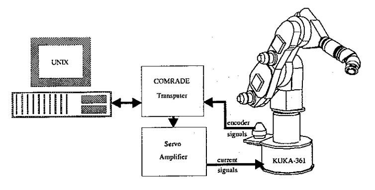
Fig. 4. The experimental set-up

the adaptive auxiliary signal to improve the system performance. The auxiliary signal \(l_{f_i}(t)\) is defined as

\[l_{f_i} = \frac{\hat{L}_{1_i}^2 \mathbf{b}_{\mathbf{m}_i} \mathbf{P}_i \mathbf{e}_{\mathbf{f}_i}}{\hat{L}_{1_i} \|\mathbf{b}_{\mathbf{m}_i}^{\mathbf{T}} \mathbf{P}_i \mathbf{e}_{\mathbf{f}_i} \| + \epsilon_i}\](32)

where

\[\hat{L}_{1_i} = \hat{\alpha}_i |\dot{x}_{p_i}| \tag{33}\] with \(\hat{\alpha}_i\) is the estimate of \(\alpha_i^*\) defined in Eq. 30 for ith force-controlled direction.

Now, substituting the control law of Eq. 31 into the error dynamics of Eq. 25 yields

\[m_{f_i}\ddot{e}_{f_i} + (b_{f_i} + \hat{k}_{vf_i})\dot{e}_{f_i} + (k_{e_i} + \hat{k}_{pf_i})e_{f_i} = k_{e_i}b_{f_i}(\dot{x}_{e_i} - l_{f_i}).\](34)

The force error dynamics given by Eq. 34 can be written in state space form as

\[\begin{bmatrix} \dot{e}_{f_{i}} \\ \ddot{e}_{f_{i}} \end{bmatrix} = \begin{bmatrix} 0 & 1 \\ -\frac{k_{e_{i}} + \hat{k}_{pf_{i}}}{m_{f_{i}}} & -\frac{b_{f_{i}} + \hat{k}_{vf_{i}}}{m_{f_{i}}} \end{bmatrix} \begin{bmatrix} e_{f_{i}} \\ \dot{e}_{f_{i}} \end{bmatrix} \\ + \begin{bmatrix} 0 \\ m_{f_{i}}^{-1} \end{bmatrix} k_{c_{i}} b_{f_{i}} (\dot{x}_{e_{i}} - l_{f_{i}}).\] (35)

Let the desired behavior of the force-tracking error for each force controlled subspace \(e_{m_i}\) is specified as

\[\begin{bmatrix} \dot{e}_{m_i} \\ \ddot{e}_{m_i} \end{bmatrix} = \begin{bmatrix} 0 & 1 \\ -\omega_i^2 & -2\xi_i\omega_i \end{bmatrix} \begin{bmatrix} e_{m_i} \\ \dot{e}_{m_i} \end{bmatrix} + \begin{bmatrix} 0 \\ 1 \end{bmatrix} 0,\] \[\dot{\mathbf{e}}_{m_i} = \mathbf{A}_{\mathbf{m}_i} \mathbf{e}_{\mathbf{m}_i} + \mathbf{b}_{\mathbf{m}_i} \mathbf{0}.\] (36)

where \(\xi_i\) and \(\omega_i\) are the desired damping ratio and undamped natural frequency of the error dynamics, respectively.

Define the tracking error state as

\[\mathbf{E_i} = \begin{bmatrix} e_{m_i} - e_{f_i} \\ \dot{e}_{m_i} - e_{f_i} \end{bmatrix} . \tag{37}\]

The proposed adaptation law to update the controller gains are given by

\[\begin{split} \dot{\hat{\vartheta}}_{i} &= -\Gamma_{i} \mathbf{b}_{\mathbf{m}_{i}}^{\mathbf{T}} \mathbf{P}_{i} \mathbf{E}_{i} \mathbf{e}_{\mathbf{f}_{i}} - \sigma_{i} \Gamma_{i} \hat{\vartheta}_{i}, \quad \hat{\vartheta}_{i}(0) > 0, \quad (38a) \\ \dot{\hat{\alpha}}_{i} &= \Gamma_{i} ||\mathbf{b}_{\mathbf{m}_{i}} \mathbf{P}_{i} \mathbf{E}_{i}|| |\dot{\mathbf{x}}_{\mathbf{p}_{i}}| - \sigma_{i} \Gamma_{i} \hat{\alpha}_{i}, \quad \hat{\alpha}_{i}(0) \geq 0. \end{split}\] \[(38b)\]

Fig. 5. Tracking of 2-D contour

Theorem 1. Consider the target impedance described by Eq. 22. If the control law Eq. 31 with adaptation law Eq. 38 is used, then the closed loop system is globally ultimately bounded.

Proof. See appendix

Note that the position-based force controller does not specify the type of the position controller. The choice of the position controller depends on the performance required. Quite often that using simple conventional controllers, e.g., independent joint PD controllers, results in an acceptable performance. However, if these simple controllers can not satisfy the desired performance, more advanced controllers such as the proposed decentralized adaptive controller presented in [10] can be applied.

6. TEST SETUP

Industrial robot. The experiments to verify the proposed controller are performed on a KUKA IR-361 industrial robot. The KUKA IR-361 robot has six degrees of freedom and is equipped with a force/torque sensor. Each of the robot axes is driven by a DC motor equipped with a digital encoder and a tachometer. The DC motor is controlled using a PI controller based on velocity (tachomenter) feedback (velocity mode). The input to these servo controllers are the desired velocities.

Force Sensor. The force sensor used in the experiments is a 6 DOF commercial force/torque sensor from Schunk which uses strain gauges measurements. The measurement range of the force/torque sensor 200 N for forces and 20 Nm for torques. Since the

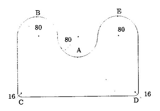
Fig. 6. Workpiece for 2-D contour tracking (radius in mm)

the contour. In this experiment, the performance of the existing position-based force controller, which consists of a fixed-gain proportional feedback, and the proposed position-based adaptive force controller given in Sec. 5 are compared.

Task specification

\(x_t\) : force controlled : \(f_{dx_t} = 25 \text{ N}\)

\(y_t\): velocity controlled:

\(\dot{y}_{d_s} = 25, 35, 45, 55 \text{ mm/s}\)

\(\alpha_{z_t}\): track (on velocities)

task frame: rotate

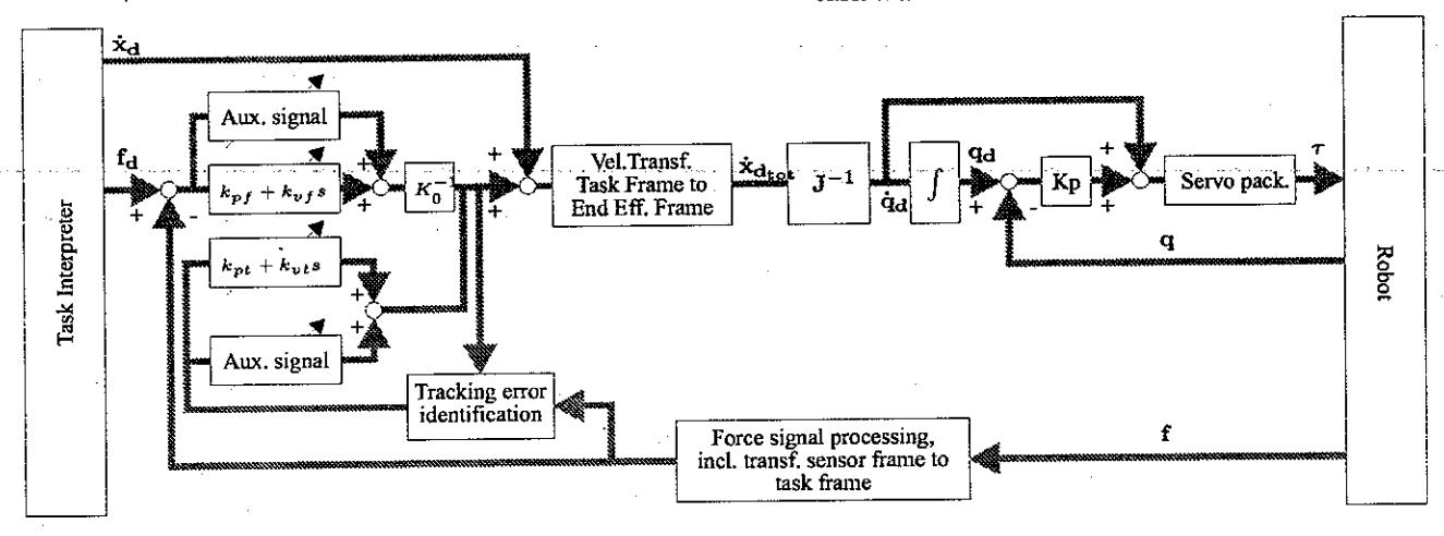
Fig. 7. Overall control scheme

force/torque measurements are noisy, digital low-pass filters with a cut-off frequency 5 Hz are applied.

Software. The proposed control schemes are implemented in the COMRADE (COmpliant Motion Research And Development Environment) which is a software package developed at PMA Div., Mech. Eng. Dept., KU-Leuven to facilitate the development and tuning of compliant motion robot tasks [24]. The software runs at a sampling rate of 120 Hz. The COMRADE environment is executed on a transputer system in a VME bus which runs under the UNIX operating system.

7. 2-D CONTOUR TRACKING

Many robot applications such as deburring, polishing, require contour following motions. In these applications the manipulator is required to apply a desired force normal to the contour while moving along the contour. In these experiments, the manipulator is required to track a 2-D contour whose geometry and location are not known as shown in Fig. 5. Figure 6 shows the geometry of the contour. The task requires the manipulator to move along the contour at constant speed while applying a constant force normal to the contour. To achieve this task the controller is required to keep the orientation of the theoretical task-frame constant with respect to

In this task, the orientation error \(\Delta \alpha_{z_t}\) is estimated on the basis of velocity measurement described in [6], and the task frame is set rotate (relative) with respect to the end-effector frame. Therefore, during the tracking motion, the orientation of the end-effector does not change with respect to the base frame.

Force control. Figure 7 shows the detailed control scheme used in the experiments. The existing force and tracking controllers are fixed P (proportional) controllers. In this experiment, the position-based adaptive force controller is applied for both force and tracking control. The existing PD controller is used for the inner controller (position controller).

The existing fixed gains of the force controller for x, y and z-directions are:

\[\mathbf{k_{pf}} = [8\ 8\ 8]\ mm/Ns,\] and the fixed tracking gains about x, y and z-axes are

\[\mathbf{k_t} = [3.25 \ 3.25 \ 3.25] \text{ rad.}\]

These controller gains are tuned experimentally.

The proposed adaptive controller to generate the desired velocity applied in this experiment is given by Eq. 31 which can be written as

\[\dot{x}_{df_i} = \hat{k}_{pf_i} e_{f_i} + \hat{k}_{vf_i} e_{f_i} + \frac{\hat{L}_{1_i}^2 \mathbf{b}_{\mathbf{m}_i} \mathbf{P}_i \mathbf{e}_{\mathbf{f}_i}}{\hat{L}_{1_i} \|\mathbf{b}_{\mathbf{m}_i}^{\mathbf{T}} \mathbf{P}_i \mathbf{e}_{\mathbf{f}_i}\| + \epsilon_i}\] (39)

where \(\hat{k}_{pf_i}\) and \(\hat{k}_{vf_i}\) are the adaptive proportional gain and the adaptive derivative gain respectively. The last term of Eq. 39 is auxiliary signal to compensate the environment uncertainty. The reference model for each force-controlled direction is given by Eq. 40 below.

\[\mathbf{A}_{\mathbf{m}_{t}} = \begin{bmatrix} 0 & 1 \\ -1 & -2 \end{bmatrix}, \mathbf{b}_{\mathbf{m}_{t}} = \begin{bmatrix} 0 \\ 1 \end{bmatrix}\] (40)

The adaptation gains of the adaptive update law Eq. 38 are:

for the force controller

\[\begin{aligned} \mathbf{\Gamma} &= \begin{bmatrix} 0.075 & 0.075 & 0.075 \end{bmatrix}, \\ \sigma &= \begin{bmatrix} 0.85 & 0.85 & 0.85 \end{bmatrix}, \\ \epsilon &= \begin{bmatrix} 5 & 5 & 5 \end{bmatrix}, \end{aligned}\] for the tracking controller

\[\Gamma = \begin{bmatrix} 0.075 & 0.075 & 0.075 \end{bmatrix},\] \(\sigma = \begin{bmatrix} 0.075 & 0.075 & 0.075 \end{bmatrix},\) \(\epsilon = \begin{bmatrix} 0.4 & 0.4 & 0.4 \end{bmatrix}.\)

All of these adaptation parameters are tuned experimentally.

Tracking results. Figure 8 - 15 show the contour following experimental results.

• For low tracking velocity, the fixed P controller behaves quite well, although, it is shown that at t = 40s and t = 60s the measured contact force is decreasing along the sharp corner of the contour (see Fig. 8). At these times the tool held by the end-effector is at the corners C and D of the contour respectively (see Fig. 6). From Fig. 9, it is shown that the average contact force is around the desired set point.
• As the tracking velocity increase (35 mm/s), the contact force using the fixed controller is further decreasing along the corners (see Fig. 10). Along the corners, the average contact force at this velocity using the proposed controller is still at the desired set point.
• As the tracking velocity reaches 45 mm/s the manipulator looses contact with the contour along the corners (see Fig. 12). At this tracking velocity, the proposed controller was still able to keep contact between the manipulator and the contour (see Fig. 13).
• As the desired tracking velocity further increased (55 mm/s), the loss of contact is getting worse. It can be seen in Fig. 14, when the manipulator got back in contact it resulted impact contact forces. As shown in Fig. 15, the

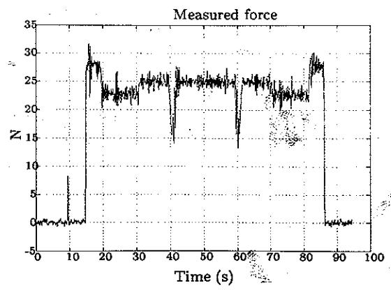
Fig. 8. Force tracking using fixed gain controller at 25 mm/s. At tracking speed 25 mm/s, the fixed P force controller is able to maintain the contact force. The contact force is decreasing along the corners C and D (t=40 s and t=60 s).

proposed adaptive controller is still able to keep contact at the corners.

It can be observed that the tracking force using the proposed position-based adaptive force controller is oscillatory. This is due to the derivative force signal, which is very noisy, applied to the force controller.

From the experiment results, it can be concluded that the proposed controller can improve the force tracking remarkably. The maximum tracking velocity is increased from 45 mm/s to 55 mm/s. The problem left for the proposed controller is the oscillation due to force derivation. In the controller implementation, the derivative force signal is obtained by filtering the measured force signal using a simple derivative filter, which is clearly not adequate. To improve the controller performance, therefore, it is required to implement an estimator in order to estimate the derivative force signal [20].

8. CONCLUSION

This paper presents robust adaptive force control for constrained manipulators. The proposed controller is developed using impedance control scheme that achieves the desired contact force by manipulating the desired position of the end-effector. The stability of the proposed controller is established using Lyapunov-based model reference adaptive control. The experiment results show that the proposed controller can improve the tracking performance remarkably.

9. ACKNOWLEDGEMENT

The first author wishes to thank, Prof H. Van Brussel and Prof J. Swevers Afdeling PMA, Werktuigkunde, KU-Leuven Belgie, for providing the possibility to do

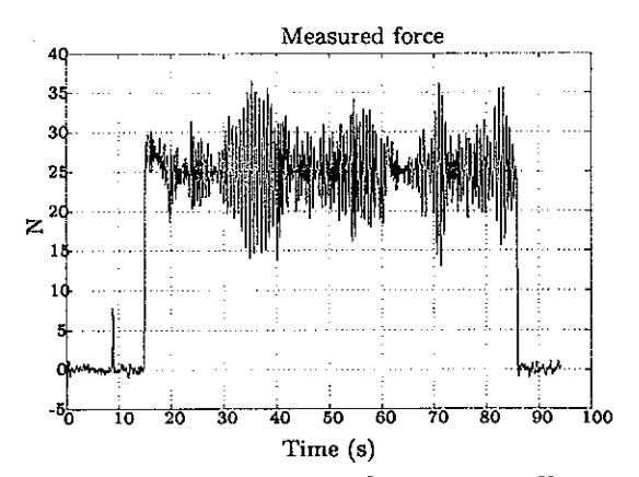
Fig. 9. Force tracking using adaptive controller at 25 mm/s. At tracking speed 25 mm/s, the proposed adaptive controller is able to keep the average contact force equal to the desired contact force along the corners C and D (t=40 s and t=60 s). The measured contact force is oscillatory due to the derivative force signal applied to the force signal.

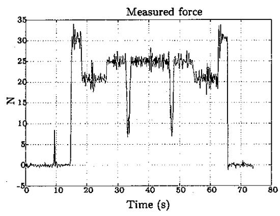
Fig. 10. Force tracking fixed gain controller at 35 mm/s. At this tracking speed, the controller is able to maintain the contact between the endeffector and the contour along the corners C and D (t=33 s and t = 47 s). However, the contact force along these corners is decreasing remarkably.

research at the PMA. This paper presents research results of the Belgian programme on Interuniversity Poles of attraction initiated by the Belgian State, Prime Ministers Office, Science Policy Programming. The scientific responsibility is assumed by its authors.