

1 Introduction
Conceptual aircraft design phase forms a critical part of the overall aircraft design processes, meaning that a decision taken in this phase has a significant impact on the technical and economic viability to the further aircraft development. In another words, any correction and change required further downstream is usually more difficult to be revised and is very costly. Therefore, decisions taken in the conceptual phase have to be close to "the best solution", i.e. "right the first time".
In conceptual design, most analyses are carried out quantitatively by applying particular mathematical expressions [1,2]. For example, the equations of aircraft geometry, aircraft performance and aircraft stability are usually represented in multivariable equations that can be expressed as explicit or implicit expressions.
The constraint propagation technique had been widely implemented in a computation for aircraft design and operations. Kuntjoro [4] explored a propagation technique for doing research on the airframe configuration design. In another research field, the application of constaint propagation in aircraft operation was excellently investigated by Gronkvist as published in [3]. In conceptual aircraft design, the implementations of constraint propagation technique carried out in [5,6], where several known design variable are propagated to suitable unknown parameters through appropriate constrains (implicit equations). So it is required to develop a logic algorithm to solve inner and outer propagations as described in Section 2. In order to illustrate the propagation through constrains, let start with a general multivariable explicit equation given as follows,
\[z = F(x, y, v, w) \tag{1}\] where, x, y, v, w : are independent variables z : is a dependent variable
F( ) : mathematical expression representing the relation between the dependent variable and the independent variables.
In sequential programming, using explicit formula is considered as the way to calculate dependent variables. Whenever it is required to compute a particular variable, then an appropriate explicit equation has to be reformed accordingly. It looks easy, just a matter of rewriting all modified parts of program. But it is not practical according to the concept of the latest software engineering and tend to prompt some errors [9,10].
Instead of requiring a user to rewrite a part of program due to some changes, it is much better to express all mathematical models in implicit forms such as shown in Equation (2). All equations are rewritten in homogeneous expression, where the symbol C is for implicit function (constraint). Unlike Equation (1), Equation (2) does not distinguish between dependent and independent variables. Marriott [7] groups the variables of constraints into two states, namely known variables and unknown variables expressed as follows,
\[C(x^k, y^u, z^k, v^u, w^u) = 0\] (2)
where, superscript k: is for known variables
superscript u: is for unknown variable
If some variables are assigned as known variables, then the logic of program searches for the first constraint that has only one unknown variable. When the selected constraint is found, the unknown variable can be computed locally by implementing a method called the local propagation. Let consider a set of three constraints namely Equation (3a), (3b), and (3c) as follows.
\[x + y^2 + \sin w = 0 \tag{3a}\]
\[\sqrt{x} + z + 5w = 0 \tag{3b}\]
\[2x + \tan y + 2v = 0 \tag{3c}\]
Suppose two variables x and z are assigned as known variables. At the first step, supposed the logic of program found Equation (3a), where there are two unknown variables in this constraint, so this constraint cannot be solved at this time. In the next step, it considers Equation (3b), where there is right only one unknown variable, namely w, to be computed by using the local propagation as explained in Section 2. The result of the local propagation is that the variable w becomes a known variable. Because all variable of Equation (3b) are already known, in the next iteration, this constraint will not be considered as the path of propagation.
By applying the three known variables, the logic of program found equation (3a), where this constraint has only one unknown variable, so the unknown variable y can be computed. As there are four known variables, the logic of program will omit Equation (3b) and then carry on to search another equation for instance Equation (3c).
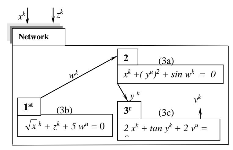
Figure 1 An illustration of network of constraint propagation
The advantage of the implementation of constraint propagation is that the computer program becomes more flexible to respond to different tasks ordered by the user. On the other hand, the disadvantages are more computing time required as every constraint has to be checked, and memory size will increase both in storage and RAM at run time. However, for a satisfaction of users, in order to increase some the flexibility of computer program, the implementation of constraint propagation is promising some benefits, where all problems of development may fall to the shoulders of software engineers.
2 The Propagation Technique
2.1 The States of Constraints
It is grouped three terminologies [5,6] for the states of constraints that are intensively used in this work. The first is the condition of over defined constraint(s), where it occurs when all variables in any constraint are assigned by user or already known, such that the constraint does not satisfy the expression of constraint as follows,
\[C(x^k, y^k, z^k, v^k, w^k) \neq 0 \tag{4}\]
In this case, the values of known variables result in an inequality (inconsistency) for the constraint (4). The user should make some changes on the set of known variables.
Secondly, well-defined constraint, it occurs when any constraint has exactly one unknown variable. For example, in Constraint (5) the unknown variable w u is ready to be calculated by using a local propagation. It results in w k as a new known variable obtained by a local propagation.
\[C\left(x^{k}, y^{k}, z^{k}, v^{k}, w^{u}\right) = 0\] \[(5)\]
Finally, under-defined constraint, it occurs when the state of constraint has more than one unknown variables. Therefore it cannot be solved directly except some unknown variables are assigned as known variables or assigned as temporary variables. For example, in constraint (6) the local propagation cannot be performed, unless v u or w u is assigned to be a temporary variable.
\[C\left(x^{k}, y^{k}, z^{k}, v^{u}, w^{u}\right) = 0 \tag{6}\]
2.2 The Local Constraint Propagation
There are three advantages of implementing a homogeneous expression. Firstly, it is expressed in the same model as in a method for solving the root of nonlinear mathematical model. Secondly, no effort needed to manipulate it into an explicit model although the unknown variable that will be calculated may be changed. The last, sometimes the constraint cannot be expressed in an explicit model such as y x2 + x y2 = 0. Hence the local propagation implemented here can govern to various mathematical models. In this work, the case study is done for the implementation of propagation for algebraic models and trigonometry models.
The logic of a local propagation can be described as follows. The first step is searching for a well defined constraint. If it is found, then the second is to identify the state of variables by examining the flag of every variable, for example in constraint (5) w is an unknown variable. In the third step, the logic calls the solver of local propagation.
The solver used for the local propagation is a numerical method described in Equation (7) and (8). The unknown variable can be computed by using a numerical method for finding roots. In this work, Newton Raphson method has been chosen for solving the computation of unknown variable. Some classical problems may arise such as multiple root finding and stability of convergence. Fortunately, in the conceptual design, most variables represent the physical properties, so the values of design variables are real and bounded to the specific ranges. So the solution of multiple roots can be handled by controlling the range of unknown variables. For example, the design variable of wing taper ratio has a range between 0 and 1.3, so the root of the equation can be localized within this interval. To illustrate the Newton Raphson method, it is given a constraint expressed as follows,
\[C\left(x^{u}, y^{k}, z^{k}\right) = 0 \tag{7}\] where.
\(x^{u}\) is the unknown variable
\(y^k\) and \(z^k\) are known variables.
Supposed, it is determined an initial value and the first increment \(\Delta x\). In order to solve the unknown variable x of Constraint (7), an iterative technique is applied to the constrain as described in [5,8]. The iteration is formed as follows,
\[x_{i+1} = x_i - \frac{C(x_i, y^k, z^k)}{C'(x_i, y^k, z^k)}\] (8)
The value of \(C(x_i, y^k, z^k)\) is computed by setting \(x = x_i, y^k\) and \(z^k\). The derivative of Constraint (7) is computed by Equation (9) as follows,
\[C'\left(x_{i}, y^{k}, x^{k}\right) = \frac{C\left(\left(x_{i} + \Delta x\right), y^{k}, x^{k}\right) - C\left(\left(x_{i} - \Delta x\right), y^{k}, x^{k}\right)}{2 \Delta x} \tag{9}\]
It can be summarized that the procedure for solving the local propagation by applying Newton Raphson method is as follows:
- a) Determine the initial unknown value of \(x = x_0\) as starting point.
- b) Determine the initial small increment \(\Delta x\)
- c) Compute the value of \(C(x_i, y^k, z^k)\) and \(C'(x_i, y^k, z^k)\)
- d) If \(|C(x_i, y^k, z^k)| \le \varepsilon\), then \(x_i\) is the root of constraint
- e) If (d) is not satisfied, then calculate \(x_{i+1}\) using Equation (8)
2.3 Inter Constraint Propagation
Figure 1 describes the propagation of known variables in the network of three constraints. It is shown that the propagation performs successfully in every constraint. However, in the constraint propagation network, the success of the propagation depends on the state of constraints. There are two possible network conditions namely adequate-defined network and under-defined network [6].
Adequate-Defined Network, the condition happens when the user assigns some known variables, so that the number constraints are adequate to propagate some known variables. For example, the condition of adequate-defined network is presented in Figure 1 where every constraint has only one unknown variable for every step. It is an ideal case in network propagation, however, most well defined network need iterations in order to solve the all unknown variables.
Under-Defined Network, it occurs when the set of constraints and the set of known variables are unable to be propagated directly, so no local propagation will never be performed unless there are assigned temporary known variables.
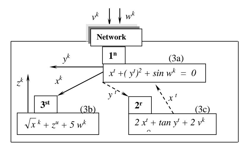
Figure 2 An example of under defined network propagation
Currently the logic of program developed in this work is only effective for the condition that the number of unknown variables is no more than two in every constraint and the number of under-defined constraints is the same as the number of unknown variables in common. Figure 2 illustrates, the example this case, there are three unknown variables and three constraints. In order to solve the unknown variable in the network, it is introduced the new status of variable namely temporary known variable. The idea is that all unknown variables are assigned with temporary within their ranges, then performed the local propagation among two constrains. In this example, two known variables are v and v and three unknown variables are v and v and three unknown variables are v and v and three unknown variables are v and v and three unknown variables are v and v and three unknown variables are v and v and three unknown variables are v and v and three unknown variables are v and v and three unknown variables are v and v and three unknown variables are v and v and three unknown variables are v and v and three unknown variables are v and v and three unknown variables are v and v and three unknown variables are v and v and v are logic of program is carried out the procedure of forward looping (also called indirect-propagation) that can be described as follows:
Step-1: Investigating constraint (3a), the condition are two unknown variables namely x and y. Therefore, at this time, there is no local propagation for this constraint, then will check the next possible constraint.
Step-2: Investigating constraint (3b), the condition is that there are two unknown variables namely x and z. Therefore, at this time, there is no local propagation for this constraint. The propagation will not perform the local constraint propagation and will check the next possible constraint.
Step-3: Investigating constraint (3c), the condition is that there are two unknown variables, namely x and y. Therefore, at this time, there is no local propagation for this constraint. The propagation will not perform the local constraint propagation and will check the next possible constraint.
Step-4: The investigation concludes that it needs to call the procedure of forward looping in order to handle temporary values. It also investigates the three unknown design variables.
Step-5: It is identified that constraint (3a) and (3c) have x and y as unknown variables and then set a flag for starting an iteration. The logic of program changes unknown variables to be temporary variables, for example a temporary variable \(x^t\). Every temporary variable acts as known variable except that its value will be changed during the iteration.
Step-6: After receiving the current value of \(x^t\), constraint (3c) is able to do a local propagation, resulting temporary value \(y^t\). In following section, constraint (3a) and constraint (3c) are called as a pair of constraints.
Step-7: Since the second iteration, constraint (3a) has \(x^t\) and \(y^t\) as temporary variables. This step has a condition, if \(|x^t + (y^t)^2 + \sin w^k| \le \varepsilon\) then they are set as \(x^k = x^t\) and \(y^k = y^t\). It means that the values of variable x and y now are not temporary but computed values (known variable), then the iteration is stopped. If the condition is not satisfied, then the value of \(x^t\) is increased until the condition is satisfied.
Step-8: After receiving the new known variables, namely \(x^k\) and \(y^k\), constraint (3b) is able to order a local propagation that result in a known variable \(z^k\)
3 Some Mathematical Models
Torenbeek [1] expresses some lifting surface and tail volume equations. In this case study [6], there six are equations to conduct as the set of constrains as described in the following equations.
Constraint 1:
\[AR - \frac{b^2}{S} = 0 \tag{10a}\]
Constraint 2:
\[C_{root} - \frac{2}{1+\lambda} \sqrt{\frac{S}{AR}} = 0 \tag{10b}\]
Constraint 3:
\[MAC - \frac{2}{3}C_{root}\left(\frac{1+\lambda+\lambda^2}{1+\lambda}\right) = 0\] (10c)
Constraint 4:
\[\tan \Lambda_{LE} - \tan \Lambda_{c/4} + \frac{0.1}{AR} \left( \frac{1-\lambda}{1+\lambda} \right) = 0\] (10d)
Constraint 5:
\[V_h - \frac{S_h l_h}{S * MAC} = 0 \tag{10e}\]
Constraint 6:
\[V_{\nu} - \frac{S_{\nu} l_{\nu}}{S*b} = 0 \tag{10f}\] where.
\(S = \text{wing area } [\text{meter}^2]\)
AR = wing aspect ratio
\(\lambda\) = wing taper ratio
\(B = \text{wing span} \quad [\text{meter}]\)
\(C_{root}\) = wing root chord [meter]
MAC = mean aerodynamic chord [meter]
\(\Lambda_{LE}\) = wing leading edge sweep angle [deg]
\(\Lambda_{c/4}\) = wing quarter chord sweep angle [deg]
\(S_h\) = area of HTP [meter<sup>2</sup>]
\(l_h\) = tail arm of HTP [meter]
\(V_h\) = tail volume of HTP [meter<sup>3</sup>]
\(S_v = \text{area of VTP [meter}^2]\)
\(l_{v}\) = tail arm of VTP [meter]
\(V_{v}\) = tail volume of VTP [meter<sup>3</sup>].
4 The Development of Computer Application
4.1 Use Case Diagram
Use case diagrams visualize the behavior of program [10], the way of user interact to the program has to be defined before going to further developments.
In this work, the application should be able to be run by a single user using personal computer. The following use case diagram is derived from four user requirements (cases). Firstly, the user should be able to get information about the idea of the constraint propagation network through a window dialog whenever it is needed. Secondly, the application should provide a window dialog where the user is able to select any or all constraints that are going to be involved in the network. Thirdly, through a window dialog, the user should be able to select which design variables are decided to be involved in the set of known variables. In addition, the dialog has to depict the range of all design variables so that the user can easily enter the value of known design variables. Finally, the user is able to execute the propagation of known design variables in the set of selected constraints. All symbols and notations applied in the use case diagram are conforming to the convention of Unified Modeling Language [10].
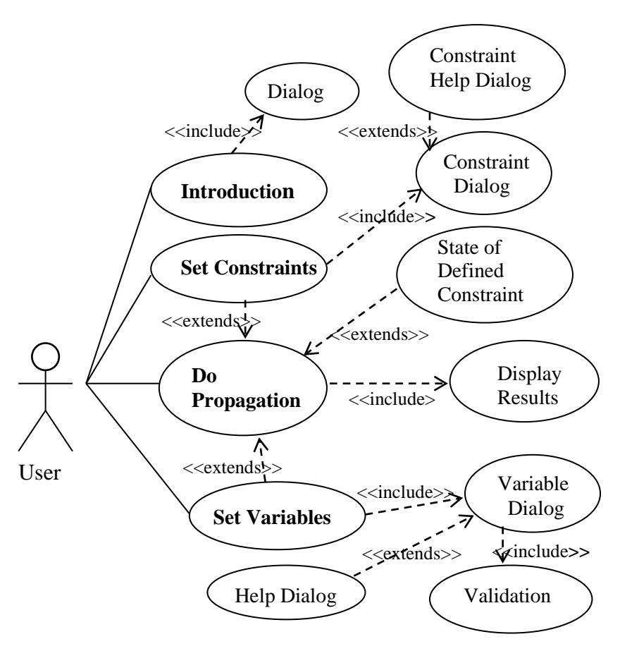
Figure 3 The use-case diagram for the constraint propagation network
4.2 Class Diagram
A class diagram becomes a truly central within an object-oriented programming [10] as it able to show a typical interaction among classes. This computer application implements three types of class relationship, namely aggregation, composition and inheritance. In the following figure, it is depicted the class diagram that will be the reference for the development of the computer code. In order to keep consistency with the convention of Visual C++, the name of every class is started by capital C.
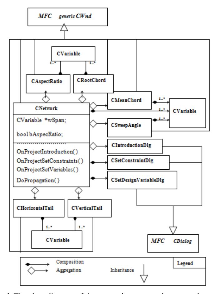
Fig.4 The class diagram of the constraint propagation network
There are eleven classes involved in the diagram, namely: CNetwork, CVariable, the six classes dealing with constraints namely CAspectRatio,
CRootChord, CMeanChord, CSweepAngle, CHorizontalTail and CVerticalTail, and the three classes dealing with dialog boxes namely CIntroductionDlg, CSetConstraintDlg and CSetDesignVariableDlg. The CVariable is considered as the base of building block, because other classes composite it in order to declare some design variables as their data members.
Another class called CNetwork is dedicated to manage the whole constraint propagation network. This class utilizes CVariable in order to create some design variables as its data members. Also, it composites CSetConstraintDlg and CSetDesignVariableDlg in order to access the selected constraints and information of the known design variables. Moreover, the class aggregates the six classes in order to have access to their member functions. In addition, it also aggregates CIntroductionDlg for accessing the introduction of the constraint propagation network. Finally, in order to inform the step of the propagation by using pop-up windows, CNetwork requires accessing some member functions of generic CWnd dealing with message boxes and dialog boxes. Therefore, CNetwork inherits a based-class called generic CWnd provided by Visual C++.
The class of CVariable acts as a basic element in the class diagram. It is used for creating all design variables of the network such as wing span, taper ratio and vertical-tail arm. The class has two types of data members i.e. value and status that are declared as public. There are four integers can be assigned for the status of variable The status (flag) are described as follows:
- status = 0 is for an unknown design variable whose value is defined in the constructor of the class.
- status = 1 is for a temporary design variable whose value is assigned to any temporary value.
- status = 2 is for a computed design variable (known variable) whose value is assigned to the result of computation.
- status = 3 is for a user-supplied design variable (known variable) whose value is assigned to the input of the user.
The computer application is developed from scratch by implementing the use case diagram and the class diagram. The main menu of the application consists of four pull-down menus, namely File, Project, View and Help. In order to fully demonstrate the capability of constraint propagation, it is provided an option for user to select independently which constraints and design variables are involved in the set of propagation.
The submenu of SetConstraints is intended to provide an option to select constraints by check box as shown in Figure 5a. The submenu of SetVariables is intended to provide the selection of the fourteen design variables. The user may select some design variables by clicking in their check boxes and then enter particular values within their range, see Figure 5b. When the user presses OK, then the application validates all the selected known design variables. After selecting the constraints and entering the design variables, the user may start the constraint propagation by selecting the submenu of DoPropagation. The application selects appropriate paths in order to perform the propagation.
Figure 5 The dialog boxes for the constraints and design variables selection
5 Testing and Evaluation
In this section, the performance of the application is tested and evaluated by applying some combination of selected constraints and known design variables. The response of the application is presented and discussed.
Case 1
Supposed that a user selects only the constraint of AspectRatio and three design variables, namely wing area, aspect ratio and wing span. Their values are entered as follows: wing area = 10 meter2 , wing span = 30 and aspect ratio = 6.5. Then the application indicates that all design variables are inside their range, but the combination of the three design variables is not satisfy (inconsistent) according to the selected constraint as shown in Figure 5.
Case 2
The application is tested to perform the indirect constraint propagation by selecting two constraints that have two unknown design variables as shown in Figure 6. By investigating the two constraints it is found that there are two unknown design variables namely wing area and wing span. When the user clicks submenu DoPropagation, firstly, the application carries out the direct
inter-constraint propagation, but none of the selected constraints performs the condition of well defined constraint. In this case, due to Equation (10a) and Equation (10f) have two unknown variables, inter constrain propagation is (flag) performing and the result of calculation is shown in Figure 6b.
Figure 6 The pair of two unknown variables
Case 3
Similar to Case 2, but currently the user selected all constraints. The application is tested to perform the indirect constraint propagation. The result of case 3 is depicted in Figure 8, where the result is similar to the case 2 shown in Figure 7. It is because no more known variables can be propagated by the rest of the four constraints.
Figure 7 The results of the indirect constraint propagation
6 Conclusion and Recommendation
6.1 Conclusions
- a) In general, the constraint propagation technique shows some flexibility to select the set of design variables and constraints. Therefore, it is promising to be implemented in conceptual aircraft design due to the need of various starting point.
- b) The Newton-Raphson method described in Section 2.2 performs an excellent solution to the local propagation. As a constraint is expressed in a homogeneous model, the solution of a constraint is treated in a similar way to solve the unknown variable.
- c) The indirect propagation is able to solve the problem of pair of constraints by using a technique of temporary known variables as shown in Case 2 and Case 3.
6.2 Recommendation
- a) In the local constraint propagation, the mathematical model applied here is algebraic and trigonometric expressions. In the next development, it is needed to implement other model like logarithmic models.
- b) In order to manage an existing file of constraints propagation such as design variables and the results of propagation, it is required to add a function for read and write in a File-menu.
7 References
- [1] Torenbeek, E., Synthesis of Subsonic Airplane Design, ISBN 90-247- 2724-3, Delft University Press, Delft, 1982
- [2] Bil, C., Development and Application of A Computer-based System for Conceptual Aircraft Design, Ph.D. dissertation, Delft University Press, Delft, 1988
- [3] Gronkvist, M., Accelerating column Generation for Aircraft Scheduling Using Constraint Propagation, Journal of Computers and Operations Research, 33(10), 2918-2934, October 2006.
- [4] Kuntjoro, W., Airframe Configuration Design Using Constraint Propagation Technique Case Wing Structure, 21st ICAS Congress, Melbourne, 13–18 September 1998.
- [5] Kolb, M.A., Constraint-Based Component-Modeling for Knowledge-Based Design, Aerospace Design Conference, Irvine, February 3-6, 1992
- [6] Zain, R., Some Applications of Constraint Propagation To Conceptual Aircraft Design In Visual C++ Environment, Master Thesis, RMIT Australia, 1999.
- [7] Marriott, K., and Stuckey, P.J., Programming with Constraint: An introduction, ISBN 0-262-13341-5, The MIT Press, Cambridge, 1998
- [8] Mooris, J.L.I, and Marriott, K., Computational Methods in Elementary Numerical Analysis, ISBN 0-471-10410-1, John Wiley and Sons Ltd., Bristol, 1983
- [9] Deitel, H.M. and Deitel, P.J., C++ How To Program, 2rd edition, ISBN 0-13-528910-6, Prentice-Hall Inc., New Jersey, 1998.
- [10] Fowler, M., and Scott, K., UML Distilled: Applying the Standard Object Modeling Language, Addison Wesley Longman Inc., Massachusetts, 1998.