

1 Introduction
Recently years, development of Micro Unmanned Aerial Vehicle for indoor application has attracted significant attention. Search and rescue in structurally unstable building, reconnaissance, surveillance of underground tunnel are examples of indoor mission in which MAVs plays an important role [0]. Compare to other MAV configurations such as fixed wing, flapping wing, conventional main/tail rotor helicopter, tandem twin rotor helicopter, coaxial rotor helicopter is properly the most suitable configuration for indoor MAV [0].
One of the typical indoor mission scenarios is to acquire an environment perception where human presence is highly risky. The vehicle shall takeoff from a place nearby, enter and explore the space, which may contain the obstacles with difference in shape and size [0]. To operate in these flying conditions, the vehicle should be equipped with certain level of autonomous control. A model based controller which derived from the mathematical is properly a good candidate for this matter. Development of helicopter dynamic model that sufficient accurate and simple enough raises a challenge to reach the full autonomous flight.
In order to obtain an appropriate dynamic model for simulation and control, a nonlinear dynamic model of micro coaxial MAV is derived from the first principle of modeling. The model is based on the physical law of aerodynamics and mechanics. Equations of motion are derived from rigid body equation in the considering of dynamic of rotary part as rotor system and stabilizer bar.
Towards the full development of dynamic model, a study on rotor performance has been carried out. The study not only aims to understand the aerodynamics of a reference platform helicopter, but also to establish a model for determining of aerodynamic force and moment of rotor system for further development. In addition, development of control system is also dealt with by the initialization of the control structure. These three issues will be introduced in turn in this article.
2 Modeling of Mathematical Model of Coaxial MAV Dynamics
2.1 Coaxial Helicopter platform
A commercial available coaxial helicopter from E Hely is used as one of the platform of the research. Main specification of this platform is represented in Table 1.
| Specification | Parameter |
| Total weight | 205 g |
| Total height | 175 mm |
Rotor diameter 340 mm
Distance between two rotors
Table 1 E Hely Specification
E Hely uses two same rotors in coaxial arrangement, one above the other. Two motor are used to drive the rotors in opposite direction, one per each. A swashplate system is mounted into the lower rotor to control longitudinal and lateral motion of the helicopter. Two servos are used to control the swashplate system through linkages to change the tilt angle of the swashplate cyclically. On upper rotor, a teetering type stabilizer bar is attached to upper rotor, and is driven at the same speed as this rotor. A control augmentation will be input into the upper rotor by cyclically change the pitch of upper rotor. Detail of reference platform and its component is depicted in Figure 1.
60 mm
Figure 1 E Hely Coaxial Helicopter
2.2 Developement of Nonlinear Analytical Mathematical Model of coaial rotor MAV
Micro coaxial helicopter is a complex nonlinear system with high order dynamics. Dynamic of coaxial helicopter is a characterized by the coupling of rotor and fuselage, rotor and stabilizer bar. Besides that, the dynamics of the helicopter in general changes over the flight condition. These features raise the difficulties in development of appropriate dynamic model.
Due to the complication of the coupling dynamics in rotor system, it is not sufficient to capture the helicopter dynamics by using only the rigid body equation of motion [0]. To precisely obtain the mathematical model, dynamics of rotor as well as its coupling dynamics will be included into the full model. Dynamic model will derived by using the basic rigid equation of motion for 6 degrees of freedom. Then, dynamics of rotor and flybar system will be added in the consideration of coupling effect. Detail of dynamic modeling process is presented in following paragraphs.
2.2.1 Coordinate Frame and Kinermatics
The system will be separated into rotors, fuselage and stabilizer bar. The two rotors are modeled as disc, located at du, dl respectively to the vehicle center of gravity. Upper rotor is turned in counter clockwise direction at rotational speed ωu, while the lower rotor rotated in clockwise at rotational speed of ωl. The corresponding thrust and torque generated by upper/lower rotor are denoted as Tu, Tl, Qu and Ql respectively.
Figure 2 Simplified Model of Reference Platform
Throughout the modeling process, two right hand coordinates are used. The first right hand coordinate is the inertia frame, denoted as O E E E x y z , , , that is fixed to the original position of the helicopter. The second one, named body fixed frame C E E E 1 2 3 , , , is fixed to the helicopter's center of gravity. Two
coordinates are relative by a transformation matrix \(R(\eta)\) that represents the orientation of body fixed frame with respect to the inertial frame [0]
\[R(\eta) = \begin{bmatrix} c_{\theta} c_{\psi} & s_{\phi} s_{\theta} c_{\psi} - c_{\phi} s_{\psi} & c_{\phi} s_{\theta} c_{\psi} + s_{\phi} s_{\psi} \\ c_{\theta} s_{\psi} & s_{\phi} s_{\theta} s_{\psi} + c_{\phi} c_{\psi} & c_{\phi} s_{\theta} s_{\psi} - s_{\phi} c_{\psi} \\ -s_{\theta} & s_{\phi} c_{\theta} & c_{\phi} c_{\theta} \end{bmatrix}\](1)
\(\eta = [\psi, \theta, \phi]\): is the yaw, pitch and roll respectively, \(c_{\alpha} = \cos \alpha\); \(s_{\alpha} = \sin \alpha\) are the short hand notations
Under this definition, transformation of velocity from body frame to inertial frame is expressed as:
\[\begin{bmatrix} \dot{x} & \dot{y} & \dot{z} \end{bmatrix}^T = R(\eta) \begin{bmatrix} u & v & w \end{bmatrix}^T \tag{2}\]
To transform the angular velocity between two mentioned coordinates, a transformation matrix is used:
\[\begin{bmatrix} \dot{\phi} \\ \dot{\theta} \\ \dot{\psi} \end{bmatrix} = \begin{bmatrix} 1 & \sin\phi \tan\theta & \cos\phi \tan\theta \\ 0 & \cos\phi & -\sin\phi \\ 0 & \sin\phi/\cos\theta & \cos\phi/\cos\theta \end{bmatrix} \begin{bmatrix} p \\ q \\ r \end{bmatrix}\] (3)
2.2.2 Rigid Body Equation of Motion
The rigid body equation of motion of micro coaxial helicopter is based on the one that is used for conventional helicopter. It is derived from Euler-Newton Equation [0]:
\[\begin{bmatrix} mI_{3x3} & 0 \\ 0 & I \end{bmatrix} \begin{bmatrix} \dot{V} \\ \dot{\Omega} \end{bmatrix} + \begin{bmatrix} \Omega \times mV \\ \Omega \times I\Omega \end{bmatrix} = \begin{bmatrix} F \\ \tau \end{bmatrix}\] (4)
where F and \(\tau\) respectively represent the vector of external forces and external torques applied to the vehicle expressed in the body fixed frame; \(I \in R^{3\times 3}\) the vehicle inertia matrix, \(V = [u, v, w]^T\) is the linear velocity vector expressed in body fixed frame and m is the total weight of the helicopter.
It is assumed that there is no coupling between the first and second term in Equation (4). Hence, the rigid body equation of motion can be rewritten in term of translational Equation (5) and rotational Equation (6):
\[m\dot{V} + \Omega \times m = F \tag{5}\]
\[I\dot{\Omega} + \Omega \times I\Omega = \tau \tag{6}\]
In calculation of torque, the torque generated by the gyroscopic effect of rotor system and flybar are also taken into account.
\[\tau_{gyro} = -\omega_u G_u \Omega - \omega_u G_f \Omega + \omega_l G_l \Omega \tag{7}\]
Where \(G_{u,l,f}\) is the skew matrix of upper, lower rotor and flybar, determined from inertia moment of rotor blade, flybar about its spinning axis \(I_{rot}\).
Full rigid body equation of motion can be expanded as:
\[\dot{u} = \frac{\left(T_{u}\right)_{X} + \left(T_{l}\right)_{X}}{m} - qw + rv - g\sin\theta\] \[\dot{v} = \frac{\left(T_{u}\right)_{Y} + \left(T_{l}\right)_{Y}}{m} - ru + pw + g\sin\phi\cos\theta\] \[\dot{w} = \frac{\left(T_{u}\right)_{Z} + \left(T_{l}\right)_{Z}}{m} - pv + qu + g\cos\phi\cos\theta\] (8)
\[\dot{p} = \frac{1}{I_{x}} \begin{bmatrix} qr(I_{y} - I_{z}) - I_{xz}pq - I_{xz}\dot{r} - \omega_{u}I_{rot-u}q - \\ -\omega_{u}I_{rot-f}q + \omega_{l}I_{rot-l}q + \tau_{x} \end{bmatrix} \dot{q} = \frac{1}{I_{y}} \begin{bmatrix} pr(I_{z} - I_{x}) + I_{xz}(p^{2} - r^{2}) + \omega_{u}I_{rot-u}p + \\ +\omega_{u}I_{rot-f}p - \omega_{l}I_{rot-l}p + \tau_{y} \end{bmatrix} \dot{r} = \frac{1}{I_{z}} \begin{bmatrix} pq(I_{x} - I_{y}) + I_{xz}qr + Q_{u} - Q_{l} \end{bmatrix}\] (9)
Where \((T_u)_X\), \((T_u)_Y\), \((T_u)_Z\), \((T_l)_X\), \((T_l)_Y\), \((T_l)_Z\), are components of thrust along the X, Y, Z axis respectively of upper and lower rotor; \(\tau_X\), \(\tau_Y\) denote the total external torque acting about the X, Y axis; \(I_X\), \(I_Y\), \(I_Z\), \(I_{XZ}\) are the inertial moments and cross product of inertia; \(I_{rot\_f}\), \(I_{rot\_u}\), \(I_{rot\_l}\) are the inertial moment of flybar, upper, lower rotor about its spinning axis.
2.2.3 Calculation of Forces and Torques
The main aerodynamic forces and torque is generated by the rotor system. In order to determine these quantities, Blade Element Momentum Theory (BEMT) is applied for two rotors in coaxial arrangement.
In coaxial rotor helicopter, the upper rotor affects to lower rotor. This effect is captured by considering the downwash from the upper rotor as an addition in vertical velocity to lower rotor. Momentum Theory will be used to calculate the magnitude of the upper rotor downwash, while the Blade Element Theory is used to determine the generated force and moment on each rotor. The calculation is done under following assumptions:
- The upper rotor is not affected by slipstream of the lower rotor;
- The lower rotor is fully affected by the upper rotor's downwash;
- Downwash direction of the upper rotor is vertical downward;
- — The position of the lower rotor is close enough to the upper rotor.
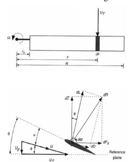
Figure 3 Element and forces
The Blade Element Theory bases on the concept that the rotor blade consists of certain number of elements. Each element is considered as an airfoil section that follows a helical path. The lift and drag are then calculated from the resultant velocity acting on the element.
Consider an element at the position r on the blade as depicted in
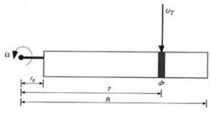
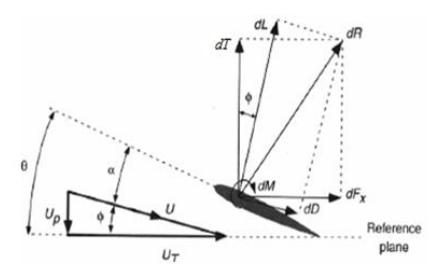
Figure 3, for a small downwash angle \(\phi\), thrust dT and torque dQ acting on a blade element at span – wise position r can be defined as [0]
\[dT = dL\cos\phi - dD\sin\phi \approx 0.5\rho U^2 c dr \left[ C_l - \phi C_d \right]\] \[dQ = r \left( dL\sin\phi + dD\cos\phi \right) \approx 0.5\rho U^2 r c dr \left[ \phi C_l + C_d \right]\] (10)
with air density \(\rho\), the lift and drag coefficient \(C_l\) and \(C_d\).
The total thrust and torque of the rotor are obtained by integrating the individual contribution of each element along the radius and multiplying by the number of blade
\[T = b \int_{r}^{R} dT \qquad Q = b \int_{r}^{R} dQ \qquad (11)\] with b is the number of rotor blade, \(r_0\) and R are the inner and outer radius of the rotor blade.
Equation (12) is used to calculate the drag coefficient. The total drag will consist of profile drag \(C_{d_0}\) and induced drag \(C_{d_i}\)
\[C_d = C_{d_0} + C_{d_0} (12)\]
It is known that the induced drag is only calculated for a finite wing. In order to determine induced drag on elements, which are considered as 2D wing, an induced drag for each element using virtual 3D effect is proposed. With this concept, the blade twist as well as the chord span-wise distribution could be taken into the aerodynamic drag force and moment calculation. The equation of total drag coefficient can be rewritten as
\[C_d = C_{d_0} + \delta_1 (\theta - \phi) + \delta_2 (\theta - \phi)^2 + C_l^2 / \pi ARe\] (13)
with e is the Oswald's factor, calculated for the whole blade by
\[e = 1.78 \left( 1 - 0.045 A R^{0.68} \right) - 0.64 \tag{14}\]
Induced velocity at the element can be determined as
\[v = \left(\frac{V_{v}}{2} + \frac{bca\Omega}{16\pi}\right) \left(-1 + \sqrt{1 + \frac{2\Omega r\left(\theta - \frac{V_{v}}{\Omega r}\right)}{\frac{4\pi V_{v}^{2}}{bca\Omega} + V_{v} + \frac{bca\Omega}{16\pi}}}\right)\](15)
where \(\Omega\) is the rotor's rotational speed, a and c are the lift slope and the chord length of the wing section.
The strongly effect of low Reynolds number combine with the customized blade section raise the difficulty for the calculation of lift and profile drag. In order to estimate these coefficients, computational fluid dynamics (CFD) is carried out for 2-dimension wing.
It is assume that the thrust vector always perpendicular to the rotor tip path plane. As the rotor disk is tilted at angle \(\beta\), thrust vector is deflected at angle \(a_{\beta}\), \(b_{\beta}\) respectively to the longitudinal and lateral axis as illustrated in
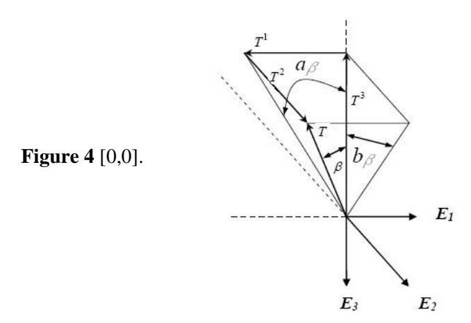
Figure 4 Rotor thrust vector
Since then, the thrust vector can be described using the two angles as Equation (16) where thrust is calculated using Equation (11).
\[\left[T_{u,l}^{X}, T_{u,l}^{Y}, T_{u,l}^{Z}\right] = \left[\frac{1}{\sqrt{1-\sin^{2}a_{\beta}.\sin^{2}b_{\beta}}}\begin{bmatrix} -\sin a_{\beta}.\cos b_{\beta} \\ \sin b_{\beta}.\cos a_{\beta} \\ -\cos a_{\beta}.\cos b_{\beta} \end{bmatrix} |T_{u,l}| \right]^{T}\] (16)
2.2.4 Dynamics of Rotor and Flybar
Dynamic of rotor acts an important role in helicopter dynamics. Rotor system creates thrust for lifting force, control force and torque, while the dynamic of rotor system is a function of control input and body motion. As a result, there is a coupling between rotor and fuselage dynamics. To include this effect, one of the properly solution is model the rotor dynamics explicitly and then couple to the fuselage equation of motion [0].
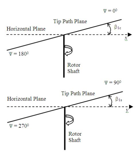
Figure 5 Longitudinal and lateral flapping of rotor
Due to the lack of flapping hinge, flapping motion of these components can be considered as the harmonic motion of teetering rotor [0]. Hence, flapping motion can be written as a function of rotor azimuth angle as
\[\beta(\psi_r) = \beta_{1c} \cos \psi_r + \beta_{1s} \sin \psi_r \tag{17}\] in which, 1 and c s are the longitudinal and lateral flapping angle.
Figure 6 Flapping angle of rotor system and flybar
Figure 6 illustrates flybar flapping angle the rotor and flybar system. To express the flapping motion, the longitudinal flapping angle and lateral flapping angle are usually used. The flapping motion is then introduced as a harmonic motion as mentioned above. Therefore, the core issue in modeling of rotor and flybar dynamics now concentrates on modeling the longitudinal and lateral motion of rotor and flybar system.
The longitudinal and lateral flapping motion of rotor system are rather complex. Rotors are high order system with the coupling effect to body dynamics. At the initial step of modeling, rotor system will be modeled as the first order system to reduce the system complicated.
Equation (18) represents the two first order differential equation that used to model the dynamic of lower rotor flapping motion. The dynamics will consist of pure rotor dynamics, coupling dynamics from the rigid body, and control input of the swash-plate system [0].
\[\dot{a} = -\frac{a}{\tau_{f,lower}} + \frac{K_b}{\tau_{f,lower}} \theta_s - \frac{A_b}{\tau_{f,lower}} b - q\] \[\dot{b} = -\frac{b}{\tau_{f,lower}} + \frac{K_b}{\tau_{f,lower}} \phi_s + \frac{B_a a}{\tau_{f,lower}} a - p\] (18)
with \(\tau_{f\_lower}\) is the time constant of lower rotor, \(\theta_s\), \(\phi_s\) are the longitudinal and lateral tilt angle of swashplate, and, \(A_b\), \(B_a\) are the cross coupling derivatives that influence the rotor flap and attitude, \(K_b\) is the ratio of swashplate tilt angle to lower rotor blade pitch angle.
In micro helicopter, a teetering type flybar is used as a secondary swashplate on upper rotor. Two bobs are attached to the bar rod at each ends; the rod is connected to the rotary shaft of upper rotor and linked to upper rotor by linkages. Due to the ability of freely rotation in vertical plane of the rod about the hinge, stabilizer bar will slow down the reaction of upper rotor by changing the rotor's pitch angle through linkages. The dynamics model of the flybar can be represented as
\[\dot{e} = -\frac{e}{\tau_{f,flybar}} + \frac{1}{\tau_{f,flybar}} \theta - q\] \[\dot{f} = -\frac{f}{\tau_{f,flybar}} + \frac{1}{\tau_{f,flybar}} \phi - p\] (19)
with the time constant of \(\tau_{f,flybar}\).
The same equation as eq. (18) is used to represent the dynamics of upper rotor. It is given as
\[\dot{c} = -\frac{c}{\tau_{f,upper}} + \frac{K_p}{\tau_{f,upper}} e - q \tag{20}\]
\[\dot{d} = -\frac{d}{\tau_{f,upper}} + \frac{K_p}{\tau_{f,upper}} f - p \tag{21}\] where \(\tau_{f\_flybar}\), \(\tau_{f\_upper}\): time constant of the flybar and upper rotor respectively. \(K_p\) is the ratio of flybar tilt angle to upper rotor blade pitch angle.
2.2.5 Full Mathematical Model
Full mathematical model is obtained by combining the rigid body dynamics, rotor system dynamics and flybar dynamics. The full dynamics model can be written in the nonlinear form of
\[\dot{X} = f(X, u) \tag{22}\] where state vector \(X = [x, y, z, u, v, w, \phi, \theta, \psi, p, q, r, a, b, c, d, e, f]\) and control input (rotational speed of rotors and tilt angles of the swashplate system) \(u = [\omega_l, \omega_u, \theta_s, \phi_s]^T\). It obviously shows that the state vector is expanded to cover the rotor dynamics in term of flapping angle.
This full dynamic model will then be used as the core mathematical model in development of simulation. An implementation of full mathematical model into Matlab Simulink will be taken place to study the performance of the helicopter.
2.3 Result and Discussion in Modeling of Coaxial Helicopter Dynamics
This section introduces the results in development of analytical mathematical of micro coaxial helicopter. Results of the study on rotor performance are first presented. Then, simulation results of a study on helicopter behavior using the analytical mathematical model are introduced.
2.3.1 Result of Study on Rotor Performance
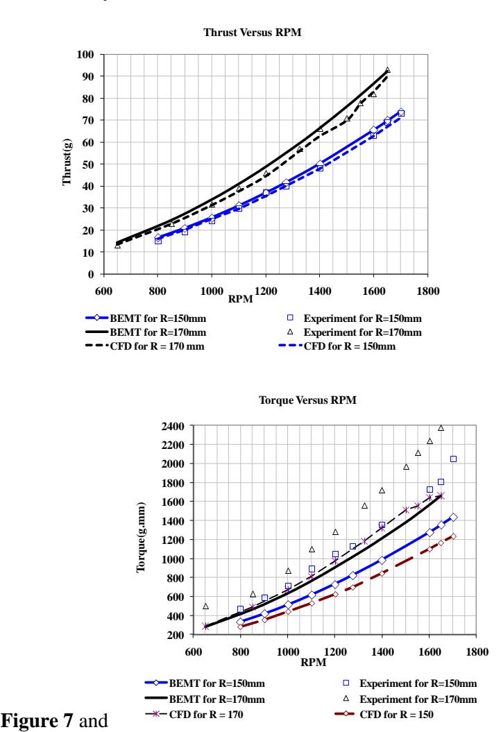
Figure 8 illustrate the result for estimation of thrust on single rotor. The results show the comparison in estimation of rotor thrust and torque using Blade Element Momentum Theory, experiment and Computation Fluid Dynamics (CFD).
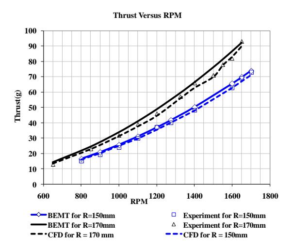
Figure 7 Estimation of force of single rotor [0]
It can be seen that the thrust estimated by BEMT is closed to the measurement value and the CFD result. The difference between the BEMT and two other approaches is between 4% and 7%. There is a quite difference in torque obtained by BEMT and experiment, CFD. However the trend of the estimation value from BEMT is quite good. Hence, it can be used to obtain the balance of torque in coaxial rotor. Detail of thrust and torque comparison is presented in Table 2.
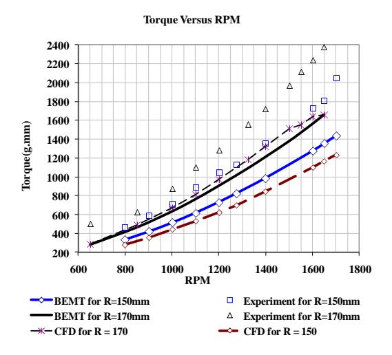
Figure 8 Estimation of torque on single rotor [0]
Table 2 Comparison in estimation of thrust and torque
| R (mm) | Pair of comparison | Average Difference (%) | |
|---|---|---|---|
| Experiment - BEMT | -4.72 | ||
| 170 | CFD - BEMT | -6.27 | |
| Experiment - BEMT | -4.06 | ||
| Thrust | 150 | CFD - BEMT | -3.84 |
| Experiment - BEMT | 44.88 | ||
| 170 | CFD(*)-BEMT(*) | 27.41 | |
| Experiment - BEMT | 39.13 | ||
| Torque | 150 | CFD(*)-BEMT(*) | 7.68 |
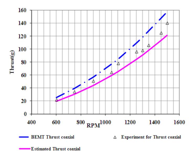
Figure 9 Estimation of thrust of coaxial rotor [0]
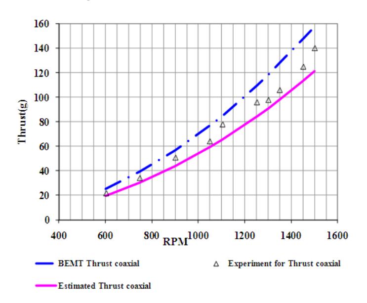
Figure 9 presents the results of estimation of thrust on coaxial rotor using BEMT, simple estimation and experiment. The calculation takes into account the interference effect between rotors. It shows that the BEMT give a higher thrust than experiment with the average different of 12.7% and standard deviation of 2.9%.
Based on above analytical and experiment results, it can be said that the rotor model using Blade Element Momentum Theory can be used to preliminary estimate the thrust and torque on single rotor and coaxial rotor.
2.3.2 Result of Study on Coaxial Helicopter Behavior
A study on helicopter behavior has been carried out based on the analytical mathematical model derived in section 0. The study aims to understand how the rotor and flybar effect to helicopter behavior [Error! Reference source not found.].
Three models of coaxial helicopter with different mathematical model are used in the study. The first model named Model 1 is the pure mathematical model of rigid body, no rotor dynamics or flybar dynamics is taken. The second model named Model 2 includes the dynamics of rotor system into the rigid body dynamics. And, the third model, Model 3, is the full dynamic model with the consideration of rotor dynamics and flybar system dynamics.
Figure 11 depicts the behavior of the helicopter due to a rolling moment disturbance. It could say that rotor and flybar dynamics have great contribution to recover the stability of the vehicle. With this contribution, the helicopter can achieve a settling attitude after the disturbance. However, a coupling motion will be resulted as a flybar is mounted on the upper rotor. There results raise the need of well understanding of rotor and flybar dynamics.
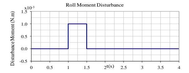
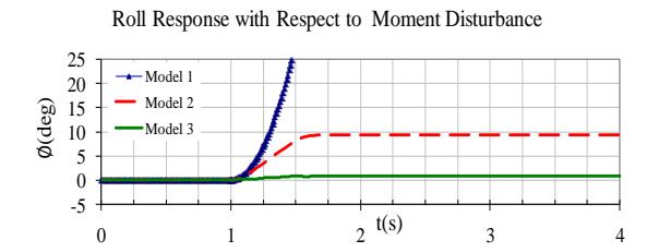
Figure 10 Response of coaxial helicopter under disturbance [Error! Reference source not found.] (con't)
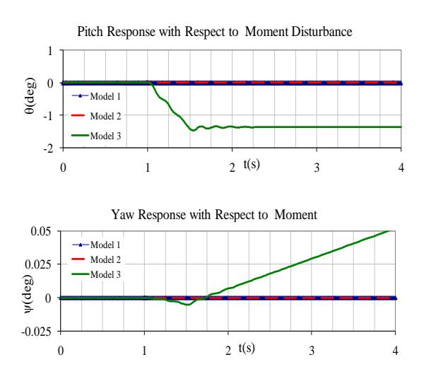
Figure 11 Response of coaxial helicopter under disturbance [Error! Reference source not found.]
3 Development of Control System
This section introduces the development of control system towards the design of hardware and software for autonomous controller.
3.1 Control System Architecture
Due to the limit payload of the MAV, only light sensors are mounted in the helicopter. The general architecture of the system is presented
Figure 12 Control system architecture
The control system consists of On Board System and the Main Processing Unit. These two systems together with the helicopter platform and the RC Console form a close system. A pair of wireless communication modules is used to transfer the data from On Board System to Main Processing Unit.
The operation of the whole system can be detailed as follows. The sensors consisted of range finder; accelerometer will collect state data of the helicopter. These data will then be packed into data package by a microcontroller. Data is finally sent to Main Processing Unit through the wireless connection.
In Main Processing Unit, a PC will be used to encode the data, which is received by the pairing wireless module. These data are then used as the input for control algorithm. A simple Altitude Hold Control Algorithm is developed and implemented to maintain the MAV altitude at desire value by varying the motor's throttle level with a determined gain. The RPM output from control algorithm is then fed to a microcontroller for generation of PWM before it is sent to helicopter through the trainer port of RC Console.
The integration On Board System, Main Processing Unit of control system can be seen in
Figure 13 System integration
Figure 14 Integration of control system into helicopter
In order to ensure the function of the control system, some ground tests have been carried out. The testing results showed that the system worked properly to the designed algorithm. The rotor RPM is increase as the altitude lower than threshold of reference altitude and vice versa; as the measure altitude is in the acceptable range, the RPM will be maintained. Typical ground test result is presented in
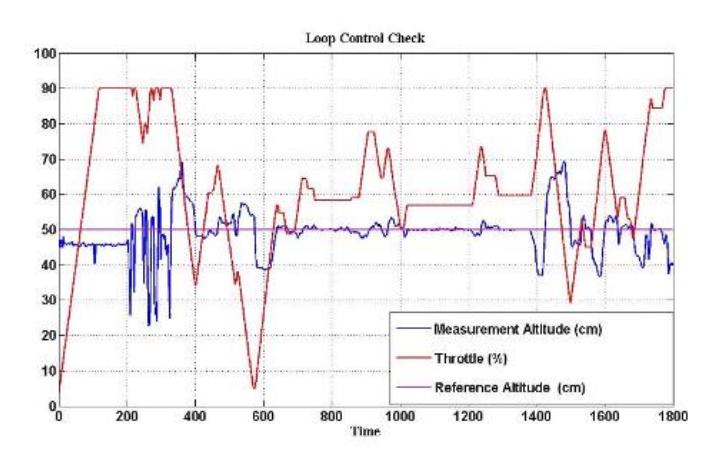
Figure 15 Result of ground testing of control system
Several flight tests have been done to verify the control system. However, it is rather difficult to obtain a stable flight because no control input is given for controlling of the attitude. Besides that, the action of the helicopter is very fast to control input. It raises the difficulty in determine of control gain to give a smooth motion.
Toward the fulfillment of the development of autonomous controller as well as the need of gathering the data for modeling of appropriate mathematical model, On Board System has been upgraded. Detail of this innovation is introduced in the next section.
3.2 Upgrade of On Board System
On Board System has been upgraded both in the quantity and quality. More sensors with appropriate accuracy are included in the sensor system to capture the necessary state of the helicopter. In the general, the method for data collecting and data processing is similar to the previous one. However, more powerful micro controller and high performance wireless connection module are used.
Upgrade On Board System consists of following sensors:
- 6DOF Inertial Measurement Unit from SparkFun Electronic, which provides the measurement of the airframe acceleration ax, ay, az and angular rate p, q, r (measure range 6g and 500deg/s, data rate: up to 200Hz);
- Digital magnetic compass (DMC) with tilt compensated OS500-S from Ocean Server for sensing heading attitude, tilt angle in longitudinal and lateral direction (resolution: 0.10 , data rate: 40Hz);
- Four Infrared Range Finder for measuring the distance from the helicopter to the obstacle in horizontal plane (range: 20-150mm);
— Sonar Range Finder sensor for measuring the helicopter altitude (range: 15cm – 6.5m)
This new onboard system could provide 6DOF helicopter state consisted of acceleration, angular rate and temporary pitch, roll attitude and heading orientation. The data update rate is 36Hz.
Figure 16 The new On Board System
4 Conclusions
In this paper the initial steps in the development of coaxial rotor helicopter are presented. As a first step, a nonlinear mathematical model is developed. The model based on the rigid body dynamics with the consideration of rotor and flybar system dynamics. An analytical model for estimation of rotor thrust and torque has been developed. Simulation with the developed dynamics model is carried out.
A control system based on the approach of PC based controller is evaluated and implemented. Two main systems are involved in the close cycle; onboard system collects data of the vehicle state; ground based is used for control and generation of control signal. A simple control algorithm is derived to maintain the altitude of the helicopter at a desired value. An upgrade has been done in the On Board System for further development.
In conclusion, it can be said that the analytical model of micro coaxial helicopter and control system have initially been developed. It showed that the dynamics model could be used for studying of helicopter behavior through the simulation. And, the control system fits not only well for coaxial rotor helicopter, but it can also be used for other configurations. On the other hand, there are still some issues need to deal with to obtain the appropriate dynamic model.
As a future work, the navigation system should be improved to capture helicopter state, including the position, attitude and velocity. In addition, parameters in the helicopter dynamic model should be identified from real flight data in a system identification process to obtain correct parameters. The last task is to expand the dynamic model of the rotor system in order to improve the whole system dynamics.
5 Acknowledgement
The authors would like to thank JICA for sponsoring the research under the Collaborative Research Program of AUNSEED-Net. The authors gratefully acknowledge the supporting from Faculty of Mechanical and Aerospace Engineering, Institut Teknologi Bandung and the Department of Aeronautics and Astronautics, The University of Tokyo.
6 Nomenclatures
| Symbol | Quantity | Units |
|---|---|---|
| x y z , , | Helicopter position in inertial x, y, z direction | |
| , , | Roll, pitch and yaw attitude respect to inertial axis | |
| u v w , , | Longitudinal, lateral & vertical velocity in body axis | m/s |
| pqr , , | Roll, pitch and yaw rate measured in body axis | rad/s |
| , s s | Longitudinal and lateral tilt of swashplate | rad |
| , u l | Rotational speed of upper and lower rotor | rad/s |
| , T T u l | Thrust generated by upper and lower rotor | N |
| , Q Q u l | Torque caused by upper, lower rotor | N.m |
| | Rotor disc tilt angle | rad |
| ab, | Rotor's longitudinal, lateral flapping angle | rad |
| m | Total vehicle mass | kg |
| ul, | Subscript of upper rotor and lower rotor | |
| T, Q | Thrust and torque | N |
| L, D | Lift and drag | N |
| Cl, Cd | Lift and drag coefficient | |
| Cf | Skin friction coefficient | |
| c | Chord length | m |
| t/c | Airfoil thickness ratio | |
| r | Span-wise position | |
|---|---|---|
| dr | Element width | m |
| r | Air density | kg/m3 |
| AR | Aspect ratio |
7 References
- [1] Sunada, S., Tokutake, H., Ohkura, A., Matsue, A., and Hirosue, W., Developing a Small, Lightweight Helicopter as a Tool Used in Everyday Life, AAIA 3rd "Unmanned Unlimited" Technical Conference, Workshop and Exhibit, Chicago, Illinois, 2004
- [2] Bouabdallah, S., Bermes, C., Schafroth, D., and Siegwart, R., "muFly: Towards a Fully Autonomous Micro Coaxial Helicopter", Full day Workshop on Micro Aerial Vehicles: Design, Control and Navigation, IROS, 2007
- [3] Mak, L. C., Kumon, M., Whitty, M., and Furukawa, T., Design and Development of The Micro Aerial Vehicle for Search, Tracking and Reconnaissance (MAVSTAR) for MAV08, MAV08 Technical Paper, 2008
- [4] Budiyono, A., Yoon, K. J., and Daniel, F. D., Integrated Identification Modeling of Rotorcraft Based Unmanned Aerial Vehicle, 17th Mediterranean Conference on Control and Automation, Makedonia Palace, Thessaloniki, Greece, 2009
- [5] Dzul, A., Hamel, T., and Lozano, R., Modeling and Nonlinear Control for a Coaxial Helicopter, IEEE International Conference on Systems, Man and Cybernetics, vol. 6, 2002
- [6] Alfred G. and Carry C M., Aerodynamics of the Helicopter, Textbook of Department of Aeronautics and Astronautics, New York University, 1967
- [7] Castillo, P., Lozano, R., and Dzul, A., Modeling and Control of Mini-Flying Machines, Springer, United State of America, 2005
- [8] Leishman, L. G., Principle of Helicopter Aerodynamics, Cambridge University Press, Cambridge, United Kingdom, 2000
- [9] Shin, J., Fujiwara, D., Nonami, K. and Hazawa, K., Model-Based Optimal Attitude and Positioning Control of Small-scale Unmanned Helicopter, Robotica, Vol. 23, 2005
- [10] Thien, H. P., Mulyanto, T., and Suzuki, S., Initial Development of a Coaxial Rotor MAV for Indoor Application, Proceeding of Joint Meeting
- Inauguration of Indonesia Section of JSME International Chapter and AUN/SEED-Net Regional Workshop on Mechanical and Aerospace, ITB, Bandung, Indonesia, 2008
- [11] Thien, H. P., Mulyanto, T., and Muhammad, H., Dynamic Modeling and Control System Development of a Coaxial Rotor MAV, Proceeding of International Forum on Strategy Technology (IFOST 2009), HoChiMinh City, VietNam, 2009