

1 Introduction
In recent years, the concept of urban air mobility (UAM) has caught immense interest. It is one big hope that having severe traffic jams, UAM can provide a faster, cleaner, and less noisy transportation service in big cities [1,2]. In the last decades, many aerospace companies have been developing such UAM, to name a few, Lilium Jet, e-Hang, and Kiti Hawk Cora [3,4]. There are many types of configurations currently developed, such as lift and cruise (L+C), lift or cruise (L/C), and lift + lift or cruise (L+L/C). These configurations correspond to various arrangements of vertical and horizontal electrical or hybrid propulsion systems as well as wing, which in general allow the UAM to perform vertical take-off and landing (VTOL), similar to helicopter, and cruise with wing, similar to conventional aircraft. Such aircraft is not only useful for reducing traffic jams, but also reaching remote areas whose access is challenging for land transportation. Not only the VTOL performance, the UAM also needs to be aerodynamically efficient, so that the energy required during cruise flight is
Diterima 5 Desember 2023, Direvisi 20 Desember 2023, Diterima untuk dipublikasikan xx Desember 2023 Copyright ©2023 Diterbitkan oleh Fakultas Teknik Mesin dan Dirgantara ITB ISSN:0852-6095, DOI: 10.5614/MESIN.2023.29.2.3
minimum. In order to attempt this, efficient wing aerodynamic performance is crucial for an aircraft.
The key to a more efficient wing aerodynamic is the shape of its airfoil. The airfoil should be designed in such a way that it produces as low drag coefficient () as possible while maintaining its lift coefficient ( ), assuming the airfoil should withstand a specific amount of aircraft weight, so that the aerodynamic efficiency (/) is minimized. In designing such airfoil, a stochastic-based optimization called genetic algorithm (GA) is one of the most popular methods to be utilized [5-9]. For example, [5] minimized the aerodynamic efficiency of aircraft with genetic algorithm, with death penalty method to handle the constraint. A drag minimization of airfoil was conducted in [6,7] with genetic algorithm as the optimizer and a class shape transformation as the shape parameterization method. The study in [8] and [9] utilized genetic algorithm to optimize multi-slat airfoil and co-flow jet airfoil, respectively.
One point to note is that since UAM utilizes propulsion system which supports vertical flights, a wing stall might be a less important aspect for UAM so that the optimized can focus on finding optimum airfoil at the design condition. Another point to note is that since the current design tends to install the propulsion system at the wing structure, the wing should not be too thin to have good structural integrity. To find such airfoil, a constrained optimization problem needs to be formulated first with the objective to minimize its drag coefficient while maintaining a reference lift and moment coefficients, with some geometrical constraints imposed.
The optimization problem is then solved by genetic algorithm with a constraint handling technique (CHT) employed. There are two types of CHTs: the conventional and the novel one. The conventional CHT, such as death penalty [10], superiority of feasible individuals (SoF)[11], favors feasible solutions over infeasible ones, which means that the infeasible solutions will always lose the selection if feasible solutions exist. Meanwhile, the novel CHT, such as generalized multiple constraint ranking [12], balances the search in both feasible and infeasible regions adaptively, in such way that some "good" infeasible solutions (infeasible solutions with better objective value than the feasible ones) are maintained during the search to enhance the process of finding optimum solution near the constraint boundaries. The promising performance of G-MCR has been shown in some previous works [12-14].
This paper aims to find an airfoil which is suitable for UAM's wing. Of course, this research is only valid for aircraft with wing installed. The optimized is genetic algorithm (GA) with two different CHTs which will be employed separately. Each GA + CHT will be run several times to ensure its consistency.
Then, the optimum airfoils obtained from the optimization are compared to a selected baseline airfoil. Deeper aerodynamic performance analysis is conducted on some best airfoils to observe their performance on the off-design conditions.
The first part of this paper presents the introduction of the problem. The second part explains the theory involved, such as general form of optimization, genetic algorithm, airfoil shape parameterization, and constraint handling techniques. Next, the third part elaborates the optimization problem definition and the optimization setting. The result and discussion are presented in the fourth part. Lastly, the fifth part concludes the current work and recommends some future works.
2 Theory
2.1 General Form of Optimization
Suppose a minimization case, an optimization can generally be formulated as follows.
Minimize \[f(\mathbf{x})\]
subject to \(g_i(\mathbf{x}) \le 0, i = 1, ..., m\)
\(h_j(\mathbf{x}) = 0, j = 1, ..., n\)
\(\mathbf{x}_L \le \mathbf{x} \le \mathbf{x}_U\) (1)
In Equation (1), \(\mathbf{x}\) denotes the d-dimensional design variable vector (d is the number of design variables). The symbols f, g, and h are the objective, inequality constraint, and equality constraint functions, respectively. The variables d, m, and n are integers. The symbols \(\mathbf{x}_L\) and \(\mathbf{x}_U\) denote the lower and upper bounds of the optimization search space, respectively.
2.2 Airfoil Shape Parameterization with Cubic B-Spline Curve
In the current work, the airfoil is parameterized with cubic B-spline curve [15]. Suppose there is a set of h + 1 control points \(P_i\), i = 0, ..., h, a cubic B-spline curve is expressed as follows,
\[\mathbf{C} = \mathbf{C}(u) = \sum_{i=0}^{h} N_{i,p}(u) \mathbf{P}_i\] (2)
where p in Equation (2) is the degree of the B-spline curve, p = 0,1,2,3. The symbol \(N_{i,p}(u)\) is the basis function, expressed as follows,
\[N_{i,0}(u) = \begin{cases} 1, & \text{if } t_i \le u < t_{i+1} \\ 0, & \text{otherwise.} \end{cases}\] (3)
\[N_{i,p}(u) = \frac{u - t_i}{t_{i+p} - t_i} N_{i,p-1}(u) + \frac{t_{i+p+1} - u}{t_{i+p+1} - t_{i+1}} N_{i+1,p-1}(u)\] (4)
where u in Equations (3) and (4) is a value between 0 and 1, and t is a set of m =h + p + 1 knots, whose expression is presented in Equations (5) to (7), as follows,
\[t_0 = t_1 = \dots = t_n = 0 \tag{5}\]
\[t_0 = t_1 = \dots = t_p = 0\] (5)
\(t_i = \frac{j}{h-p+1}, j = 1, \dots, h-p\) (6)
\[t_{m-p} = t_{m-p+1} = \dots = t_m = 1 \tag{7}\]
The shape generation of an airfoil with cubic B-spline curve is illustrated in Figure 1 (red curve). The number of control points is h + 1 = 9. The first control point \(P_0\) is set at the trailing edge. The next control points are placed in clockwise direction sequentially from the lower surface \((P_1, P_2, P_3)\), leading edge \((P_4)\), upper surface \((P_5, P_6, P_7)\), and then go back to the trailing edge \((P_8)\). The control points at trailing edge \((\mathbf{P}_0, \mathbf{P}_8)\) are fixed at \(\mathbf{x} = [1,0]^T\), while at leading edge \((\mathbf{P}_4)\)is fixed at \(\mathbf{x} = [0,0]^T\). The other control points are set active so that moving those control points will obtain different shapes of airfoil. To ensure that the leading edge of airfoil is at \([0,0]^T\), a rotation and dilatation of the red airfoil is required. The rotation to ensure that the chord of red airfoil is horizontal is conducted as follows,
\[x_r(u) = 1 + (x(u) - 1)\cos(\pi - \alpha) - y(u)\sin(\pi - \alpha)\] (8)
\[y_r(u) = (x(u) - 1)\sin(\pi - \alpha) + y(u)\cos(\pi - \alpha)\] (9)
The x(u) and y(u) in Equations (8) and (9) are the coordinates of the red curve, respectively. The \(x_r(u)\) and \(y_r(u)\) are the rotated coordinates, and \(\alpha\) is the angle between the chord line of the red airfoil and line \(P_0P_4\). Next, \(x_r(u)\) and \(y_r(u)\) are dilated to \(x_d(u)\) and \(y_d(u)\) (see Equations (10) and (11), respectively) to ensure that the leading edge of airfoil is at \([0,0]^T\) with the following process,
\[x_d(u) = \frac{x_r(u) - x_r(u)|_{@LE}}{L} \tag{10}\]
\[x_{d}(u) = \frac{x_{r}(u) - x_{r}(u)|_{@LE}}{L}\] \[y_{d}(u) = \frac{y_{r}(u) - y_{r}(u)|_{@LE}}{L}\] (10)
where \(x_r(u)|_{@LE}\) and \(y_r(u)|_{@LE}\) are the coordinates of the red airfoil's leading edge and L is its chord length.
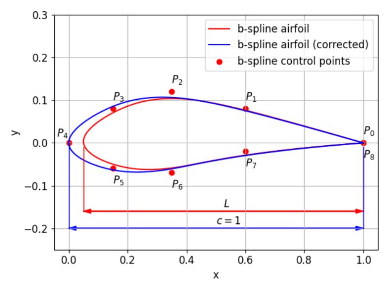
Figure 1 Illustration of airfoil shape generation with cubic B-spline curve.
2.3 Genetic Algorithm (GA)
Genetic algorithm [11] works based on the following iterative steps:
- 1. Initialize a parent population of individuals,
- 2. Evaluate the fitness value of each individual in the parent population,
- 3. Compute a stopping criterion. If it is met, then stop, else, go to Step 4,
- 4. Conduct parental selection, crossover, and mutation on parent population and generate offspring population consisting of individuals,
- 5. Evaluate the fitness value of each individual in the offspring population,
- 6. Conduct environmental selection to obtain new parent population of individuals for the next generation, then go to Step 3.
2.4 Constraint Handling Technique (CHT)
Genetic algorithm was originally developed to solve unconstrained optimization problems. Therefore, a constraint handling technique (CHT) needs to be applied in case of constrained problem. In this paper, two penalty-based techniques are considered and compared, namely superiority of feasible individuals (SoF) [11] and generalized multiple constraint ranking (G-MCR) [12].
2.4.1 Superiority of Feasible Individuals (SoF)
SoF [11] is one of the most popular CHTs which has been used in many engineering applications. It is expressed in Equation (12) as follows,
\[F(\mathbf{x}) = \begin{cases} f(\mathbf{x}), & if \ CV(\mathbf{x}) = 0, \\ f_{worst} + CV(\mathbf{x}), & otherwise. \end{cases}\](12)
where \(f_{worst}\) is the worst objective value of feasible individual in the current population and is set to zero in case there is no feasible individual. This CHT highly favors feasible individuals during the search, in such way that the infeasible individuals will always lose to feasible individuals during the selection process.
2.4.2 Generalized Multiple Constraint Ranking (G-MCR)
The G-MCR is expressed in Equation (13) as follows,
\[F(\mathbf{x}) = \beta R_f + (1 - \beta) \gamma \sum_{i=1}^m \alpha_i R_{\nu_i}\] (13)
where \(R_f\) and \(R_{\nu_i}\) are the ranks built by the queue of the individuals' objective values and the i-th constraint violation values, respectively, in the current population. The coefficient \(\beta\) the search of unconstrained optimum and feasible solutions. The coefficient \(\alpha_i\) represents the proportion of the i-th constraint to be explored during the search. Lastly, the coefficient \(\gamma\) controls the proportion between objective terms with the constraint terms. In this paper, the G-MCR formulation is based on the optimum settings found in [12], which is the G-MCR-C_9, whose coefficients are presented in Table 1.
Table 1 Coefficients of G-MCR.
| Coefficient | β | \(\alpha_i\) | γ |
|---|---|---|---|
| Value | [· (- 1)2 | \(N_{viol_i}\) | 1 |
| \(\sqrt{1-(\zeta-1)^2}\) | \(\overline{N_{pop}}\) | \(\overline{\sum_{i=1}^{m} \alpha_i}\) |
The symbol \(N_{viol_i}\) denotes the number of solutions violating the i-th constraint in the current population. The coefficient \(\zeta = \frac{N_{feas}}{N_{pop}}\), where \(N_{feas}\) is the number of feasible individuals in the current population. In principle, the G-MCR works quite differently compared to SoF. Instead of favoring feasible individuals, G-MCR tries to balance the search between feasible and infeasible regions, in the hope that the optimum solution can be found faster.
3 Experimental Setup
3.1.1 Problem Definition
The optimization problem is to minimize the drag coefficient \((C_d)\) of a two-dimensional airfoil by changing \(\mathbf{x}\), where \(\mathbf{x}\) is the design variable comprising airfoil shape and angle of attack (AoA), defined as follows,
Minimize \[C_d(\mathbf{x})\] (14) subject to \(g_1(\mathbf{x}) = \left| C_{l_{ref}} - C_l(\mathbf{x}) \right| - \varepsilon \le 0\) \(g_2(\mathbf{x}) = \left| C_m(\mathbf{x}) - C_{m_{ref}} \right| - \varepsilon \le 0\) \(g_3(\mathbf{x}) = E_x \le 0\) \(g_4(\mathbf{x}) = E_y \le 0\) \(\mathbf{x}_L \le \mathbf{x} \le \mathbf{x}_U\)
In Equation (14), the airfoil shape \(\mathbf{x}\) is parameterized with the cubic B-spline curve, using a total of nine control points as explained in Subsection 2.2. The control points at the leading and trailing edges are set to fixed, while the others are set to active. The lower and upper bounds of flexibility of the control points are presented in the first 18 rows of Table 2.
The constraints \(g_1\) and \(g_2\) are aerodynamic constraints, which is required so that while minimizing the drag coefficient, the lift and moment coefficients of the candidate optimum airfoil are around the same (within sn=0.001 difference) with the baseline airfoil's lift and moment coefficients. The constraints \(g_3\) and \(g_4\) are structural constraints to ensure that the airfoil shape is sensical geometrically. The \(g_3\) ensures the x-coordinates of the airfoils are within 0 and 1, expressed in Equation (15) as follows,
\[E_{x} = \sum_{i=1}^{N+1} e_{x_{i}} \tag{15}\] where \(e_{x_i} = |-x_i|\) if \(x_i < 0\) and \(e_{x_i} = x_i - 1\) if \(x_i > 1\), and N is the number of panels forming the airfoil. The \(g_4\) ensures that the y-coordinates of upper surfaces are not lower than the y-coordinates of the lower surfaces, expressed in Equation (15) as follows,
\[E_{y} = \sum_{i=2}^{\frac{N}{2}-1} e_{x_{i}} y_{i} - y_{i}\] (15)
where \(e_{y_i} = y_{N+1-i} - y_i\) if \(y_{N+1-i} - y_i < 0\) and \(e_{y_i} = 0\) otherwise.
The selected baseline airfoil in this paper is NACA 2412. While there is no reference to what airfoil is usually used for the UAM's wing, NACA 2412 is selected since visually, it looks to have sufficient thickness to withstand the weight of the propulsion system. Of course, further assessment with regards to its structural performance is required.
The aerodynamic coefficients are calculated with XFOIL [16], a panel methodbased airfoil aerodynamic solver which is suitable for low Reynolds Number () (the order of is around 105 to 106 ) and low subsonic flight speed. This solver is deemed suitable for the case considered in this paper because recent designs of UAMs are often in a comparable size with regular helicopters. Therefore, they most likely have low Reynolds number (reference length from the mean aerodynamic chord) and flight speed around Mach number 0.1 to 0.3.
| Design Variables | Lower Bound 𝒙𝑳 | Upper Bound 𝒙𝑼 | ||
|---|---|---|---|---|
| 𝑷0,x | 1 | 1 | ||
| 𝑷1,x | 0.8 | 0.9999 | ||
| 𝑷2,x | 0.4 | 0.7999 | ||
| 𝑷3,x | 0.0001 | 0.3999 | ||
| 𝑷4,x | 0 | 0 | ||
| 𝑷5,x | 0.0001 | 0.3999 | ||
| 𝑷6,x | 0.4 | 0.7999 | ||
| 𝑷7,x | 0.8 | 0.9999 | ||
| 𝑷8,x | 1 | 1 | ||
| 𝑷0,y | −0.0013 | −0.0013 | ||
| 𝑷1,y | −0.1 | −0.1 | ||
| 𝑷2,y | −0.1 | −0.1 | ||
| 𝑷3,y | −0.1 | −0.1 | ||
| 𝑷4,y | 0 | 0 | ||
| 𝑷5,y | 0.1 | 0.1 | ||
| 𝑷6,y | 0.1 | 0.1 | ||
| 𝑷7,y | 0.1 | 0.1 | ||
| 𝑷8,y | −0.0013 | −0.0013 | ||
| AoA (degree) | 0 | 6 | ||
Table 2 Lower and upper bounds of the design variables.
3.1.2 Optimization Setting
In minimizing the drag coefficient of airfoil, a real-coded genetic algorithm with an elitist scheme [11] is utilized. The number of solution evaluations with XFOIL is set to 10,000, which is equivalent to a population size of 100 and number of generations to 100 in the GA setting. The parent selection is conducted with binary tournament selection [17]. Regarding the crossover, the simulated binary
crossover (SBX) method [18] with distribution index of 20 and a crossover probability of one are utilized. For the mutation, polynomial mutation method [19] with distribution index of 20 and a mutation probability of 1 are utilized.
4 Result and Discussion
The optimum solutions from all three independent runs for all CHTs are presented in Table 3. The table shows that in general, all optimum solutions successfully satisfy all constraints. Regarding the objective values, the optimum solutions of all three runs of SoF (SoF_OPT_1, SoF_OPT_2, and SoF_OPT_3) cannot produce better aerodynamic characteristics from the baseline airfoil. On the other hand, the optimal solutions of all three runs of G-MCR (G-MCR_OPT_1, G-MCR_OPT_2, and G-MCR_OPT_3) can produce decrease of drag coefficient from 15.7% to 17.5%, or increase of aerodynamic efficiency (⁄) from 18.4% to 21.4%. This indicates that the airfoil can provide 18.4% to 21.4% more efficient flight on cruise flight phase with lift coefficient around 0.4.
The poor performance of SoF is most probably due to the very strict constraints imposed by the optimization problem. The constraints 1 and 2 are very close to equality constraints, which significantly increases the difficulty in obtaining feasible individuals. From random search of 10,000 random solutions within the lower and upper bounds, there is no feasible solution found, which is equivalent with 0% of the total evaluations. This situation could be one reason why the SoF, which favors feasible individuals over infeasible individuals, faces difficulties in generating better solutions. Meanwhile, G-CMR can consistently find better solutions than the baseline, indicating that balancing the search from both feasible and infeasible regions is more effective in finding better individuals in this airfoil optimization problem.
Table 3 Aerodynamic characteristics of baseline and obtained optimal airfoils (Re=1x10⁶ , M=0.1).
| Airfoil | AoA (deg.) | 𝑪𝒅 | 𝑪𝒍 | 𝑪𝒎 | 𝑳⁄𝑫 | %∆𝑪𝒅 | %∆(𝑳⁄𝑫) |
|---|---|---|---|---|---|---|---|
| Baseline | 1.499 | 0.00561 | 0.4 | -0.0486 | 71.3 | - | - |
| SoF_OPT_1 | 2.344 | 0.00783 | 0.4006 | -0.0479 | 51.16 | +39.6 | -28.2 |
| SoF _OPT_2 | 3.282 | 0.01356 | 0.4009 | -0.0477 | 29.56 | +141.7 | -58.5 |
| SoF _OPT_3 | 1.856 | 0.00788 | 0.3999 | -0.0491 | 50.75 | +40.5 | -28.8 |
| G-MCR_OPT_1 | 2.246 | 0.00463 | 0.4007 | -0.0484 | 86.54 | -17.5 | +21.4 |
| G-MCR_OPT_2 | 2.231 | 0.00473 | 0.3993 | -0.0494 | 84.42 | -15.7 | +18.4 |
| G-MCR_OPT_3 | 2.339 | 0.00468 | 0.3998 | -0.0495 | 85.43 | -16.6 | +19.8 |
The geometries of optimum airfoils obtained by GA with G-MCR as well as the baseline airfoil are presented in Figure 2. It is observed that the upper surface of the optimum airfoils tends to have smaller thickness and further back location of the maximum thickness compared to the baseline. This shape tends to reduce the pressure near the leading edge, thus reducing the drag coefficient. However, the higher curvature towards the trailing edge tends to produce earlier stall condition, thus reducing the maximum angle of attack. As for the lower surface, the optimum airfoils tend to have higher thickness with further back location of maximum thickness to produce the high-pressure component to the y-direction required to maintain its lift and moment coefficient.
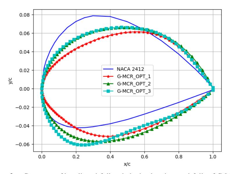
Figure 2 Geometry of baseline airfoil and obtained optimum airfoils of G-MCR.
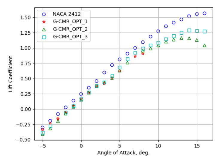
Figure 3 Lift coefficient against angle of attack of baseline airfoil and obtained optimum airfoils of G-MCR.
A deeper analysis is conducted on the optimum airfoils based on the performance along a series of angles of attack. Observing Figure 3, all optimum airfoils are found to have smaller lift coefficients for the same values of angles of attack compared to the baseline airfoil. Moreover, they also stall earlier with lower maximum lift coefficient compared to the baseline airfoil. Airfoil G-CMR_OPT_1 produces a very high drag coefficient starting from angle of attack of 7 deg., indicating that the range of operation of this airfoil is very narrow. In fact, the aerodynamic assessment of airfoil G-MCR_OPT_1 could not converge at some points, probably due to stall, so the scatter plot is incomplete.
Observing Figure 4, all optimum airfoils have a localized area near the optimized drag coefficient values. Even though the drag coefficients are the smallest at their corresponding optimal angle of attack (see Table 3), the drag coefficient immediately increases after the angle of attack either decreases or increases. This is an indication that the performance of these optimum airfoils is not robust. When there is an angle of attack disturbance (either increase or decrease), the aerodynamic efficiency of the optimum airfoils will decrease immediately.
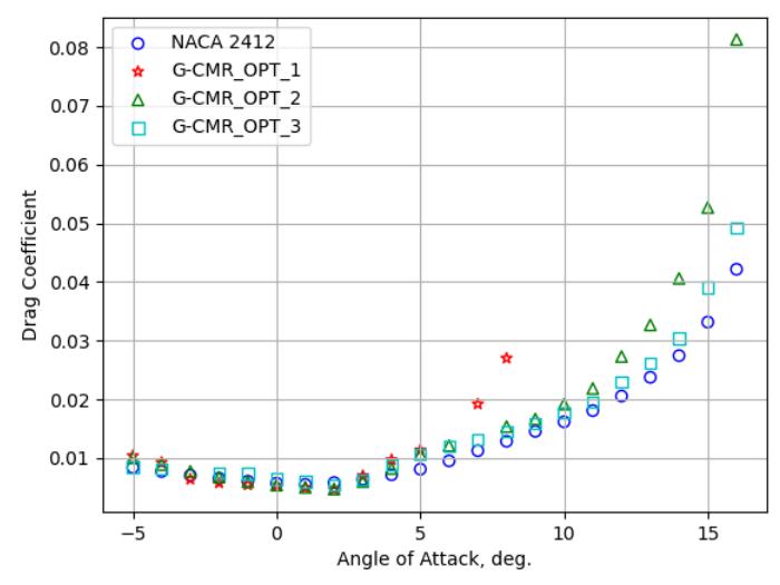
Figure 4 Drag coefficient against angle of attack of baseline airfoil and obtained optimum airfoils of G-MCR.
5 Conclusion and Future Works
Drag minimization of low subsonic airfoil has been conducted by utilizing genetic algorithm (GA) applied with two different kinds of constraint handling techniques (CHTs), namely SoF and G-MCR. From three independent runs of each CHT in GA, it was observed that G-MCR, a CHT with balanced search between feasible and infeasible regions tends to obtain better optimum airfoils than SoF, a conventional one highly favoring only feasible region. The obtained optimum airfoils can increase the aerodynamic efficiency from 18.4% to 21.4%. However, these optimum airfoils are not robust to angle of attack disturbance because a small increase or decrease of angle of attack will decrease the aerodynamic efficiency immediately. Therefore, robust optimization needs to be conducted in the future to obtain an airfoil which is not sensitive disturbances of important parameters, including but not limited to angle of attack disturbance.
6 References
[1] Rothfeld, R., Straubinger, A., Fu, M., Al Haddad, C. & Antoniou, C., Urban air mobility. In Demand for Emerging Transportation Systems, Elsevier, 267-284, 2020.
- [2] Straubinger, A., Rothfeld, R., Shamiyeh, M., Büchter, K.D., Kaiser, J. & Plötner, K.O., An overview of current research and developments in urban air mobility–Setting the scene for UAM introduction, Journal of Air Transport Management, 87, article number 101852, 2020.
- [3] Bacchini, A. & Cestino, E., Electric VTOL configurations comparison, Aerospace, 6(3), pp. 26, 2019.
- [4] Babu, M.N.P., Basa, S., Duba, P.K. & Rajalakshmi, P., Future Mobility with eVTOL Personal Air Vehicle (PAV): Urban Air Mobility (UAM) Concept, in International Conference on Electrical and Electronics Engineering, Saad Mekhilef, pp. 323-337, 2022.
- [5] Wu, M.Y., Yuan, X.Y., Chen, Z.H., Wu, W.T., Hua, Y. & Aubry, N., Airfoil shape optimization using genetic algorithm coupled deep neural networks, Physics of Fluids, 35(8), 2023.
- [6] Akram, M.T. & Kim, M.H., CFD analysis and shape optimization of airfoils using class shape transformation and genetic algorithm—Part I. Applied Sciences, 11(9), pp. 3791, 2021.
- [7] Dina, A., Danaila, S., Pricop, M.V. & Bunescu, I., Using genetic algorithms to optimize airfoils in incompressible regime, INCAS Bulletin, 11(1), pp.79-90, 2019.
- [8] Kumar, K., Kumar, P. & Singh, S.K., Aerodynamic Performance Optimization of Multiple Slat Airfoil based on Multi-Objective Genetic Algorithm, Arabian Journal for Science and Engineering, 46, pp. 7411- 7422, 2021.
- [9] Jiang, H., Xu, M. & Yao, W., Aerodynamic shape optimization of co-flow jet airfoil using a multi-island genetic algorithm, Physics of Fluids, 34(12), 2022.
- [10] Kramer, O., A review of constraint-handling techniques for evolution strategies. Applied Computational Intelligence and Soft Computing, 2010, pp.1-19, 2010.
- [11] Deb, K., An efficient constraint handling method for genetic algorithms. Computer methods in applied mechanics and engineering, 186(2-4), pp. 311–338, 2000.
- [12] Dwianto, Y.B., Fukumoto, H. & Oyama, A., Adaptively preserving solutions in both feasible and infeasible regions on generalized multiple constraint ranking, in Proceedings of the 2020 Genetic and Evolutionary Computation Conference, Joze A Lozano, pp. 690-698, 2020.
- [13] Dwianto, Y. B., Palar, P. S., Zuhal, L. R. & Oyama, A., On the Advantages of Searching Infeasible Regions in Constrained Evolutionary-Based Multi-Objective Engineering Optimization, Journal of Mechanical Design, 146(4), 2024.
- [14] Dwianto, Y.B., Fukumoto, H. & Oyama, A., Adaptively Enhancing Infeasible Region Exploration on Multiple Constraint Ranking, Transaction of the Japanese Society for Evolutionary Computation. 11(2), pp 18-28, 2020.
- [15] Bartels, R.H., Beatty, J.C., & Barsky, B.A., An introduction to splines for use in computer graphics and geometric modeling, Morgan Kaufmann, 1995.
- [16] Drela, M., XFOIL: An analysis and design system for low Reynolds number airfoils, in Low Reynolds Number Aerodynamics: Proceedings of the Conference Notre Dame, Thomas J. Mueller, pp. 1-12, 1989.
- [17] Blickle, T. Tournament selection, Evolutionary computation, 1, pp.181- 186, 2000.
- [18] Deb, K. & Agrawal, R.B., Simulated binary crossover for continuous search space, Complex systems, 9(2), pp. 115–148, 1995.
- [19] Deb, K. & Deb, D., Analysing mutation schemes for real-parameter genetic algorithms, IJAISC, 4(1), pp. 1–28, 2014.