Abstrak

Dari data sekunder dan perhitungan dimensi, gelombang laut mempunyai karakteristik fraktal. Bentuk fraktal dari gelombang laut diasumsikan mempunyai hubungan langsung dengan ketidaklinearan dari gelombang laut. Untuk pembuktian asumsi ini diambil data pengamatan 40 data seri waktu yang diambil dari eksperimen refraksi di Grays Harbor, Washington tahun 1999. Data ini dibagi menjadi 2 grup, grup pertama adalah data yang diambil di perairan dengan kedalaman 25 meter dan grup kedua diambil dari data yang diambil di perairan dengan kedalaman 12 meter. Pengambilan data di grup kedua adalah sedemikan rupa sehingga data ini adalah berasal dari gelombang yang berjalan dari data grup pertama. Setelah dilakukan perhitungan dimensi kurva dengan menggunakan Analisa Rescaled Range dan mengambil parameter Goda sebagai ukuran ketidaklinearan gelombang laut, didapati bahwa bentuk fraktal gelombang laut berhubungan langsung dengan ketidaklinearan gelombang.

1. Introduction

The word 'fractal' was coined by Mandelbrot (1983) from the Latin fractus, meaning broken. Fractal geometry is observed in many natural phenomena. In this work, we will concentrate on the fractal character of waves. Munzenmayer (1993) found that near breaking surface water waves exhibit fractal geometry. An important feature of these waves is that their surface is not continuous, and thus, non-differentiable. From field observation, we hypothesized that fractals are also related to the degree of nonlinearity of the water waves. Knowledge of whether waves are fractal motivates future research on characterizing beaches by its waves fractal number.

To introduce the concept of fractals, we consider a curve existing in a space. We measure the length of the curve by joining a series of line segments, each of length δ, end to end along the curve. The number of segments needed to traverse the curve for a given segment length δ is called the measure M ^δ. If we choose a smaller δ, then the measure M ^δ increases. The concept of dimension is defined by the relationship between M ^δ and δ as δ approaches zero:

\[M_{\delta} = \delta^{-s} \tag{1}\] where s is defined to be the dimension of the curve. To illustrate this concept, let us consider Figure 1. For the straight line segment in Figure1, evidently and the dimension of the line in Figure 1 is ¹ M^{δ δ−} =

Catatan : Usulan makalah dikirimkan pada April 2003 dan dinilai oleh peer reviewer pada tanggal 7 Mei 2003 – 2 Juni 2003. Revisi penulisan dilakukan antara tanggal 2 Juni 2003 hingga 25 September 2003.

¹⁾ Faculty at Ocean Engineering Program, Department of Civil Engineering, Bandung Institute of Technology (ITB).

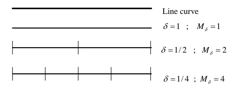
Figure 1. Line segments traversing a line curve

one.

Next, we consider complex curve shown in Figure 2. For such a curve, M \(_{\delta} = \delta^{-s}\), where 1< s <2. When a curve's dimension is non-integer, the curve is called fractal and the dimension is called the fractal dimension. This concept can be generalized to higher dimensions. For instance, for a surface, we can construct a measure by covering the surface with squares of side \(\delta\). The number of squares is the measure M \(_{\delta}\), and the relation \(M_{\delta} = \delta^{-s}\) still defines the dimension of the surface. A fractal surface would have 2 < s < 3. A graphical way to describe

\[\log M_{\delta} = -s \log \delta\] dimension is to take the logarithm of Equation (1). to obtain

We see that -s is the slope of a plot of log M \(\delta\) verse \(\log \delta\).

2. Rescaled Range Analysis

The most important method used to determine whether a set has a fractal structure is measuring its dimension. The method of rescaled range analysis is used to determine fractal dimension of a set with x and y axes not having the same physical dimension, such as free surface in y-axis and time in x-axis (Vanouplines, 1995). For example, the curve plotted in Figure 3 is a time series of free surface taken at Grays Harbor, WA in 1999. This is an example of a curve where the physical dimension in x and y are different. Hurst (1965) developed rescaled range analysis as a statistical method to analyze time series of natural phenomena. There are two parameters used in this analysis. The range R is the difference between the minimum and maximum of the cumulative sum \(X(t,\tau).X(t,\tau)\)\(\tau\)).represents the cumulative sum of measurement of some quantity \(\xi\) made at discrete time t over a total time \(\tau\). S denotes the standard deviation of the measurement \(\xi\).. We use the Benoit V1.2 \(\frac{R}{c} = (c \ \tau)^H\) Fractal Analysis software to calcu-

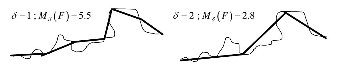
Figure 2. Measurement \(M_{\delta}\) of a curve using various line segments \(\delta\)

Where H is the Hurst exponent. The coefficient c is taken to be 0.5 by Hurst. R, S, \(\xi\), and X are formally defined as

\[R(\tau) = \max X(t, \tau) - \min X(t, \tau)\] (4)

\[S(\tau) = \sqrt{\left(\frac{1}{\tau} \sum_{t=1}^{\tau} \left\{ \xi(t) - \left\langle \xi \right\rangle_{\tau} \right\}^{2} \right)}\] (5)

where

\[\left\langle \xi \right\rangle_{\tau} = \frac{1}{\tau} \sum_{t=1}^{\tau} \xi(t) \tag{6}\]

\[X(t,\tau) = \sum_{u=1}^{t} \left\{ \xi(u) - \left\langle \xi \right\rangle_{\tau} \right\} \tag{7}\]

This method is appropriate for time series. The graphical representation uses time on the \(\chi\) axis, and the free surface elevation on the ordinate.

The Hurst exponent H has a value of about 0.72 for many natural phenomena. For ocean wave data, it is found to be between 0.12 - 0.5. The relationship between the Hurst exponent and the fractal dimension is simply (Vanouplines, 1995)

\[D = 2 - H \tag{8}\]

A Hurst exponent of 0.5 < H < 1 corresponds to a time series with trending behavior. A Hurst exponent of 0 < H < 0.5 indicates non-trending, oscillatory behavior. The oscillatory behavior has a rather high fractal dimension (1.5 < D < 2), corresponding to a highly variable time series with large standard deviation. Figure 3 shows ocean wave data measured at Gravs Harbor, Washington, in 1999. The water depth was 25 meters. The fractal dimensions calculated using rescaled range analysis is 1.756. So it is confirmed that ocean waves are fractals.

3. Goda Nonlinearity Parameter

Goda (1985) used skewness as a measure of the nonlinearity of waves. The skewness \(\sqrt{\beta_1}\) of a time series \(\eta_i\) is defined as

\[\sqrt{\beta_{1}} = \frac{1}{\eta_{rms}^{3}} \frac{1}{N} \sum_{i=1}^{N} (\eta_{i} - \eta_{mean})^{3}\] (9)

where

\[\eta_{mean} = \frac{1}{N} \sum_{i=1}^{N} \eta_i \tag{10}\] and

\[\eta_{rms} = \sqrt{\frac{1}{N} \sum_{i=1}^{N} \eta_i^2} \tag{11}\]

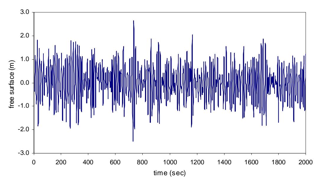
Figure 3. Free surface time series burst # 500, taken at Grays Harbor, WA in 1999. The data sampling is 2 Hz. (Gelfenbaum, et.al. (1999))

Goda also proposed a parameter describing the extent of wave nonlinearity.

\[\Pi = \frac{H_s}{L_A} \coth^3 k_A h \tag{12}\]

Goda found that the skewness of the data increases as the degree of nonlinearity increases. The dispersion relation is written as

\[\omega^2 = g \ k_A \tanh k_A h \tag{13}\] and

\[k_A = \frac{2\pi}{L_A} \tag{14}\]

H, h, \(\omega\) and k_A are the significant wave height, water depth, wave frequency, and wave number, respectively. Significant wave height H_s is the average of the highest one-third of the wave.

4. Sensitivity Test

To determine the sample size needed to obtain robust estimate of fractal dimension, a sensitivity test of fractal dimension to sample size was performed. The method of rescaled range analysis is used to determine the fractal dimension of ocean wave data taken in Sandy Duck, North Carolina in 1997. The sampling rate was 2 Hz. The raw signal is shown in Figure 4. Figure 5 summarizes the sensitivity test.

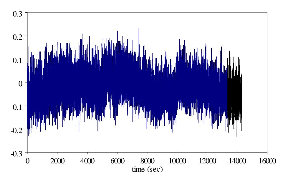
Figure 4. Ocean wave data, dt = 0.5 sec taken from Sandy Duck, North Carolina, 1997 (Courtesy of Prof Rob Holman, Oregon State University, USA)

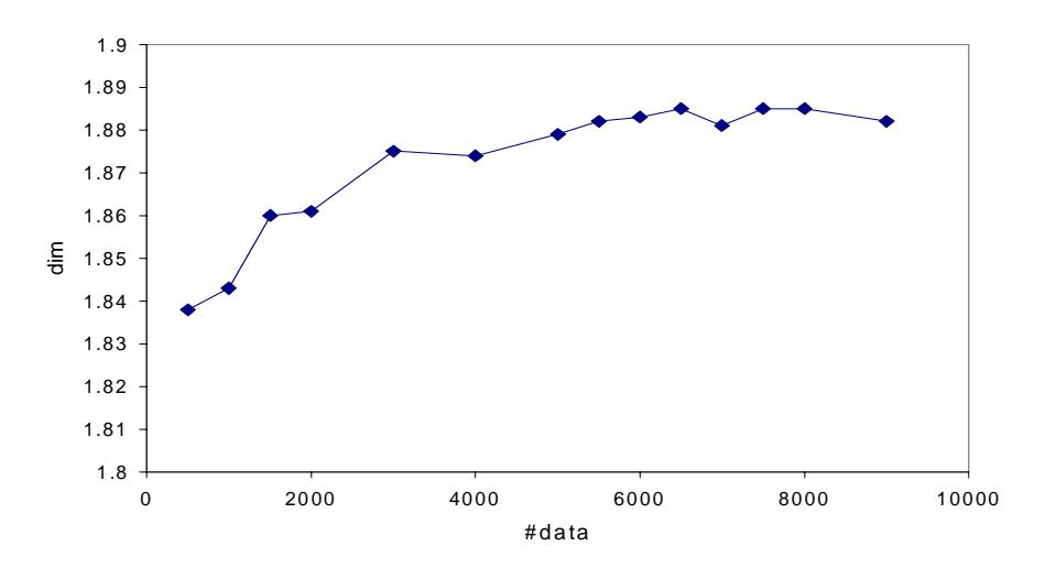
Figure 5. Average fractal dimension for different number of data blocks of ocean wave data

From Figure 5, there is little improvement in the estimated dimension for record length above 5000 datapoints. We choose to use record lengths of 4000 data in our calculations.

5. Determination of Relation Between Fractals and Nonlinearity of The Waves

Next, we consider wave data from the Grays Harbor Wave Refraction Experiment (Gelfenbaum et.al., 2000). The data are divided into two groups of 20 records, one group consists of data taken at 25 meters water depth, the other at 12 meters water depth. We selected the data with the timing subsequent to each other, counting for the estimated traveling time between location of 25 meters to 12 meters. The objective of the data analysis is to observe the relationship of fractal dimension with water depth and the degree of nonlinearity. Nonlinearity is estimated using both skewness and Goda's nonlinearity parameter. A plot of skewness verse nonlinearity parameter (Figure 6) shows the 12 meters data to have higher skewness and nonlinearity parameter values than the 25 meters data: the shallow waves are clearly more nonlinear.

Fractal dimension verse skewness is plotted in Figure 7. The fractal dimension increases as the skewness increases. Figure 8 shows that the fractal dimension also increases with increasing nonlinearity. These results indicate a strong positive correlation between fractal dimension and nonlinearity

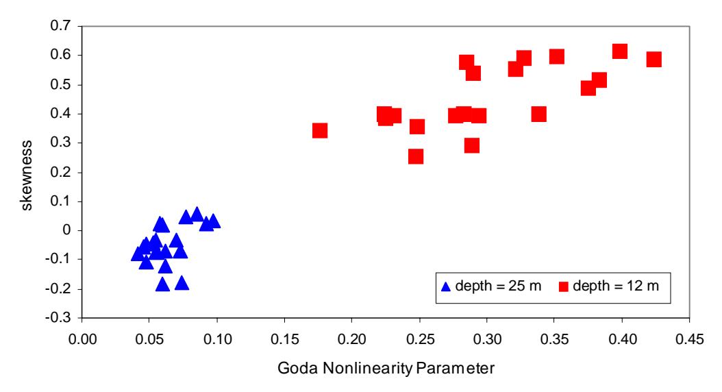
Figure 6. Skewness of surface elevation versus wave non-linearity parameter defined in the data is taken from Grays Harbor, WA

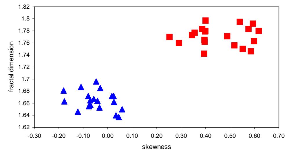
Figure 7. Fractal dimension of surface elevation versus the skewness of the statistical distribution

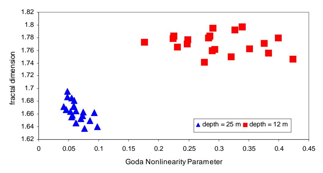
Figure 8. Fractal dimension of surface elevation versus the Goda nonlinearity parameter

6. Conclusion

From the above results, we can conclude that fractal waves have a direct relationship with the nonlinearity of the waves. The higher fractal dimension of the waves indicates higher degree of the waves nonlinearity. Figures 6 and 8 show that waves at shallow water are more non-linear than waves at deeper water. The nonlinearity of waves at the shallow water is partly due to the effect of the ocean bottom, and interactions of infragravity waves such as crosswaves, edge waves to the gravity waves that we are observing now. Turbulence effects, breaking waves may also contribute to the waves nonlinearity at the shallow water. More thorough observation is needed to validate the effects of turbulence and breaking waves.

7. Acknowledgement

The research has been funded partly by Indonesian Cultural Foundation at New York and International Student Scholarship at the Oregon State University, Corvallis.