
1. Introduction
In a seismic hazard analysis, one of the critical factors is the determination of attenuation relations. There have been a number of attenuation relations derived in the last two decades by using multi-regression analysis. Most of them were derived in a certain region where peak ground acceleration records had been available.
In this paper, the attenuation relationship for subduction zone interface and intraslab earthquakes at rock sites will be employed based on the Artificial Neural Networks (ANN) approach. Artificial Neural Network, a "new" computational paradigm, provides a fundamentally different approach to predict the ground motion. In this approach the attenuation relationship is not obtained by developing mathematical models, but it is obtained directly from existing record of ground motions data at a site using the self-organizing capabilities of the neural network. The main benefits in using an ANN approach are that all behaviors can be represented within a unified
environment of a neural network and that the network is built directly from existing data. The network is presented with the data and "learns" it relationships. Therefore, there is no a priori assumption about the system behavior.
2. Artificial Neural Networks
2.1 Architecture
Neural networks are massively parallel computational models for knowledge representation and information processing. As their name implies, neural networks are inspired by the neuronal architecture and operation of the human brain as shown in Figure 1. Because of their fundamental hardware similarity to that of the human brain, neural networks have some unique capabilities in information processing. Neural networks are the first computational models with true learning and knowledge acquisition capabilities. Neural networks can either learn from examples or
Catatan : Usulan makalah dikirimkan pada 25 Oktober 2004 dan dinilai oleh peer reviewer pada tanggal 16 Desember 2004 – 21 Desember 2004. Revisi penulisan dilakukan antara tanggal 7 Desember 2004 hingga 19 Pebruari 2004.
1. Geotechnical Engineering Laboratory, Institut Teknologi Bandung.
they can learn by interacting with their environment. Neural networks are capable of learning complex nonlinear relationships and associations from a large body of data. A neural network consists of a number of interconnected processing elements, commonly referred to as neurons. The neurons are logically arranged into two or more layers as shown in Figure 2, and interact with each other via weighted connections.
The scalar weights determine the nature and strength of the influence between the interconnected neurons. Each neuron is connected to all the neurons in the next layer. There is an input layer where data are presented to the neural network, and an output layer that holds the response of the network to the input. It is the intermediate layers, also known as hidden layers, which enable these networks to represent and compute complicated associations between inputs and outputs.
Figure 1. Biological neural networks [Fausett, 1994]
Figure 2. Typical neural networks architecture
2.2 Back-propagation algorithm
The neural networks paradigm adopted in the study utilizes the back-propagation algorithm by Rumelhart et al. [1986]. The basic mathematical concepts of the back-propagation algorithm are found in the literature [Hertz et al. 1991; Haykin 1994; Fausett 1994]. Neural networks are "trained" essentially by the presentation of a series of example patterns of associated input and target or expected output values. Each hidden and output neuron processes its inputs by multiplying each input by its weight, summing the product, and then processing the sum through a non-linear transfer function to produce a result. The sigmoid curve is commonly used as the transfer function. The neural network "learns" by modifying the weights of the neurons in response to the errors between the actual output values and the target output values. This is carried out through a gradient-descent strategy that minimizes the overall error of all the outputs neurons. One pass through the set of training patterns along with the updating of the weights is called a cycle or epoch. Training is performed by repeatedly presenting the entire set of training pattern (updating the weights at the end of each cycle) until the average sum squared error over all the training patterns is minimizes and within the tolerance specified for the problem.
Figure 3. Back-propagation process
At the end of the training phase, the neural network should correctly reproduce the target output values for the training data, provided that the errors are minimal, i.e., that convergence occurs. The associated trained weights of the neurons are then stored in the neural network memory. In the next phase, the testing phase, the trained neural network is fed a separate set of data. The neural network predictions (using the trained weights) are compared to the target output values to assess the ability of the neural network to produce (generalize) correct responses for the testing patterns that only broadly resemble the data in the training set. No additional learning (weight adjustment) occurs during this phase. Once the training and testing phases are found to be successfully, the neural network can then be put to use in practical applications. The neural network will produce almost instantaneous results of the output for the inputs provided. The predictions should be reliable, provided that the input values are within the range used in the training set. Part of the back-propagation algorithm information in this subsection was compiled from Goh [1996].
3. Reviews on The Current Attenuation Relations
Several attenuation relations have been proposed by many researchers. In general, they are categorized according to tectonic environment (i.e. subduction zone and shallow crustal earthquakes) and site condition. In this paper, several attenuation relations, which are commonly used, will be compared and described briefly as follows.
3.1 Crouse [1991]
This attenuation can be used for magnitude range from 5.0 to 9.5 and epicenter distance until 200 km. This attenuation given by the following expression:
\[Ln(Y) = 6.36 + 1.76M - 273Ln(R + 1.58 \exp(0.60M)) + 0.0091 \cdot h\]
\(\sigma = 0.773\)
Where M = moment magnitude; R = closest distance (km); h = focus depth (km).
3.2 Fukushima & Tanaka [1992]
This attenuation can be used for both subduction and shallow crustal earthquake with short to moderate distance (not greater than 300 km) the equation is:
\[\log(A) = 0.42 \cdot M_w - \log(R + 0.025 \cdot 10^{0.42M_w}) - 0.0033 \cdot R + 1.22 - 0.14 \cdot L\] \[\sigma_{logA} = 0.210\]
Where A = maximum earthquake acceleration (cm/sec<sup>2</sup> or gals). For Japanese data, L = 0, while L = 1 is used for non-Japanese data.
The equation above can be used for medium to hard soil according to Japanese soil classification.
3.3 Youngs et al. [1997]
This relation considers two types of subduction zone earthquakes, i.e. interface earthquake and intraslab earthquake. Subduction zone interface earthquakes are shallow angle thrust events that occur at the interface between the subducting and overriding plates, while intraslab events occur within subducting oceanic plate and are typically high angle; normal faulting events responding to downdip tension in the subducting plate. Attenuation relations for rock and deep soil are given as follows respectively:
\[\begin{split} &\ln(y) = 0.2418 + 1.414 M + C_1 + C_2 (10 - M)^3 + C_3 \\ &\ln(r_{rup} + 1.7818 \cdot \mathrm{e}^{0.554 M}) + 0.00607 \cdot H + 0.3846 \cdot Z_t \\ &\sigma_{\ln Y} = C_4 - C_5 \cdot M \end{split}\]
Where, y is spectral acceleration (g); M, moment magnitude; \(r_{rup}\), closest distance to rupture (km); H, depth (km); \(Z_T\), source type, 0 for interface, and 1 for intraslab.
3.4 McVerry et al. [1998]
This attenuation has been considering earthquake mechanism (i.e. crustal, subduction and dipping slab). The equation is:
\[\begin{split} Log~(PGA) &= 0.298.M - 1.56.log~(r^2 + 19^2)^{0.5} + 0.00619 \\ h_c &- 0.365 + 0.107\delta_{REV} - 0.186~\delta_{ROCK} - 0.124\delta_{INTER} \end{split}\]
Where d = 19 km is additive constant found by fitting the data, h = centroid depth (km), \(\delta_{REV} = 1\) crustal reverse mechanism, 0 for other earthquake, \(\delta_{ROCK} = 1\) for rock site, 0 for other site condition \(\delta_{INTER} = 1\) for interface event, 0 for other tectonic type.
3.5 Si & Midorikawa [2000]
It developed for short to moderate distance (less than 200 km). The earthquake classified into three kinds, i.e. crustal, interplate and intraplate earthquake. The equation for soil site is:
\[\label{eq:log_A} \begin{array}{l} Log~A = 0.50 M_W - log(X + 0.0055.10^{0.5 Mw}) - 0.003.X \\ + 0.0036.h + 0.60 + d \end{array}\]
\[\sigma_{logA} = 0.250\]
Where A = peak ground acceleration (cm/dt<sup>2</sup>), X closest distance to fault rupture (km), h focus depth (km), d = 0 for crustal, 0.09 for interplate and 0.28 for intraplate earthquake
For rock site, divided by 1.4.
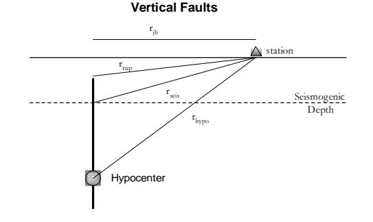
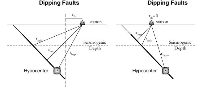
Figure 4. Source to site distance measures for attenuation models
4. Ann-Based Attenuation Relationships
4.1 Data collation and normalization
In this phase, the data was used in this study were drawn from actual peak ground acceleration compiled by Youngs [1997] for subduction zone earthquakes at the rock sites. The data was also used by Youngs to derive his attenuation relation. Ninety-nine of these PGA records were used as input in the study, ninety data for interface earthquakes and nine data for intraslab earthquakes. Details of the range of the data are summarized in Table 1. All of PGA data were used as shown in Figure 5.
To normalize inputs the preprocessing function was used in this neural network analysis. This enhances the fairness of training by preventing an input with large magnitudes from swamping out another, equally important, but smaller, input. For all iteration of the network the input is modified by the following formula.
\[xi' = (xi - (maxi + mini) / 2) / (maxi - mini).\]
This form of preprocessing calculates the maximum and minimum values for each of the inputs over the training set. The maximum and minimum for each input are stored as weights for the input layer of the network.
4.2 Derivation of attenuation relation
Since the relationships between input-output in the ANN is represent by weights, ANN-based attenuation
Table 1. Summary of range of values
| Parameters (1) | Symbol (2) | Range of Values (3) |
|---|---|---|
| Moment Magnitude | M | 5.0 – 8.0 |
| Focal depth (km) | H | 11 - 105 |
| Distance (km) | R | 12.9 – 473.4 |
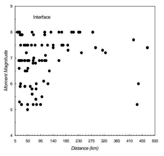
(a)
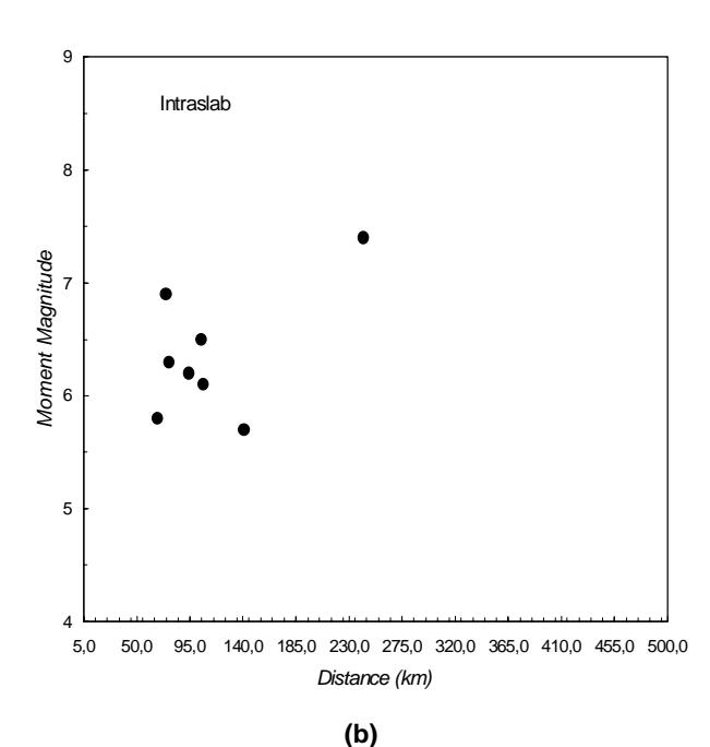
Figure 5. Distribution of PGA data set, (a) Interface, (b) Intraslab
relation in ANN equation form could be represented by the following equation:
PGA = PGA NN (H, M, R : 3 | 3 | 1), for intraslab earthquakes, and
PGA = PGA NN (H, M, R : 3 | 20 | 20 | 1), for interface earthquakes.
The symbol NN is introduced by Ghaboussi [1990] to denote the output of a multi layer feed forward ANN, and second argument field in the parentheses describes the network architecture that includes the number of neurons in each layer and the training history of the hidden layers. H is focal depth in km, M is moment magnitude and R is distance in km.
From this equation, we can see that network architecture for intraslab earthquake have 3 (three) input nodes, 3 (three) hidden nodes in one layer, and 1 (one) output node. And for interface earthquake, the network architecture have 3 (three) input nodes, 20 (twenty) hidden nodes in two layers, and 1 (one) output node. The network architecture was determined by trial and error method and several training process until specified tolerance of 0.001 reached.
In mathematical equation, proposed attenuation relation for intraslab earthquakes can be written in the following equation, i.e.:
\[y = \frac{1}{1 + e^{-\left(1.3103 - 0.8796 \frac{1}{1 + e^A} + 0.8456 \frac{1}{1 + e^B} - 6.0979 \frac{1}{1 + e^C}\right)}}\] with
A = -0.889416 - 0.007106H + 0.445802M - 0.006015R
B = 1.064208 + 0.025430H - 0.491388M + 0.004162R
C = -3.011306 - 0.006236H + 1.000046M - 0.046827R
Mathematical form of interface earthquakes being developed.
4.3 Comparison with other attenuation relations
The proposed attenuation relation is compared with other attenuation relations. The results in Figure 5 and Figure 7(a) to Figure 7(g) show less scatter in data points in comparison to other attenuation relations. The root of residual mean square, \(\sigma^2\) (i.e the sum of squares of the differences between the observed and the predicted ln PGA or Log PGA divided by degree of freedom number of equation) is also taken to evaluate variability and fitness the proposed attenuation compared with the other ones. The result is shown in the Table 2.
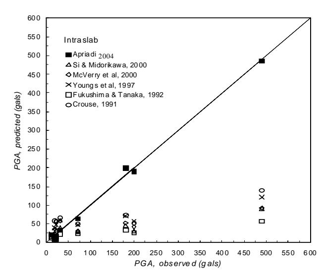
Figure 6. Comparison of PGA predicted by several attenuation relations for intraslab earthquakes
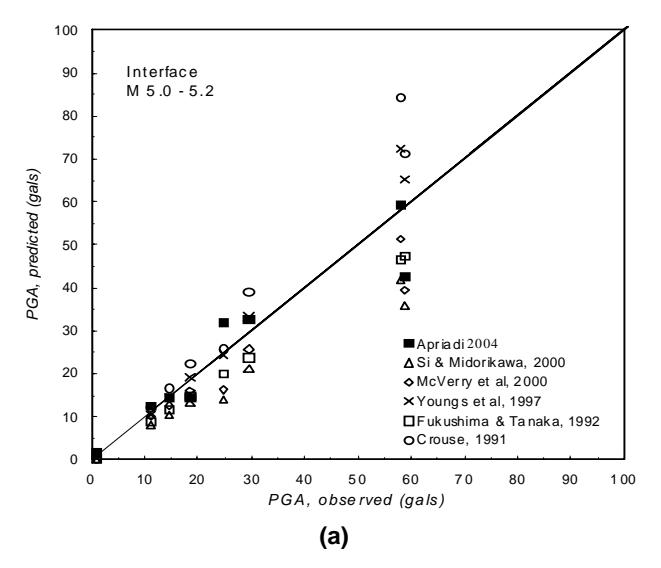
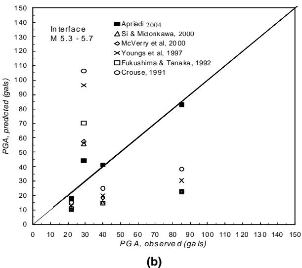
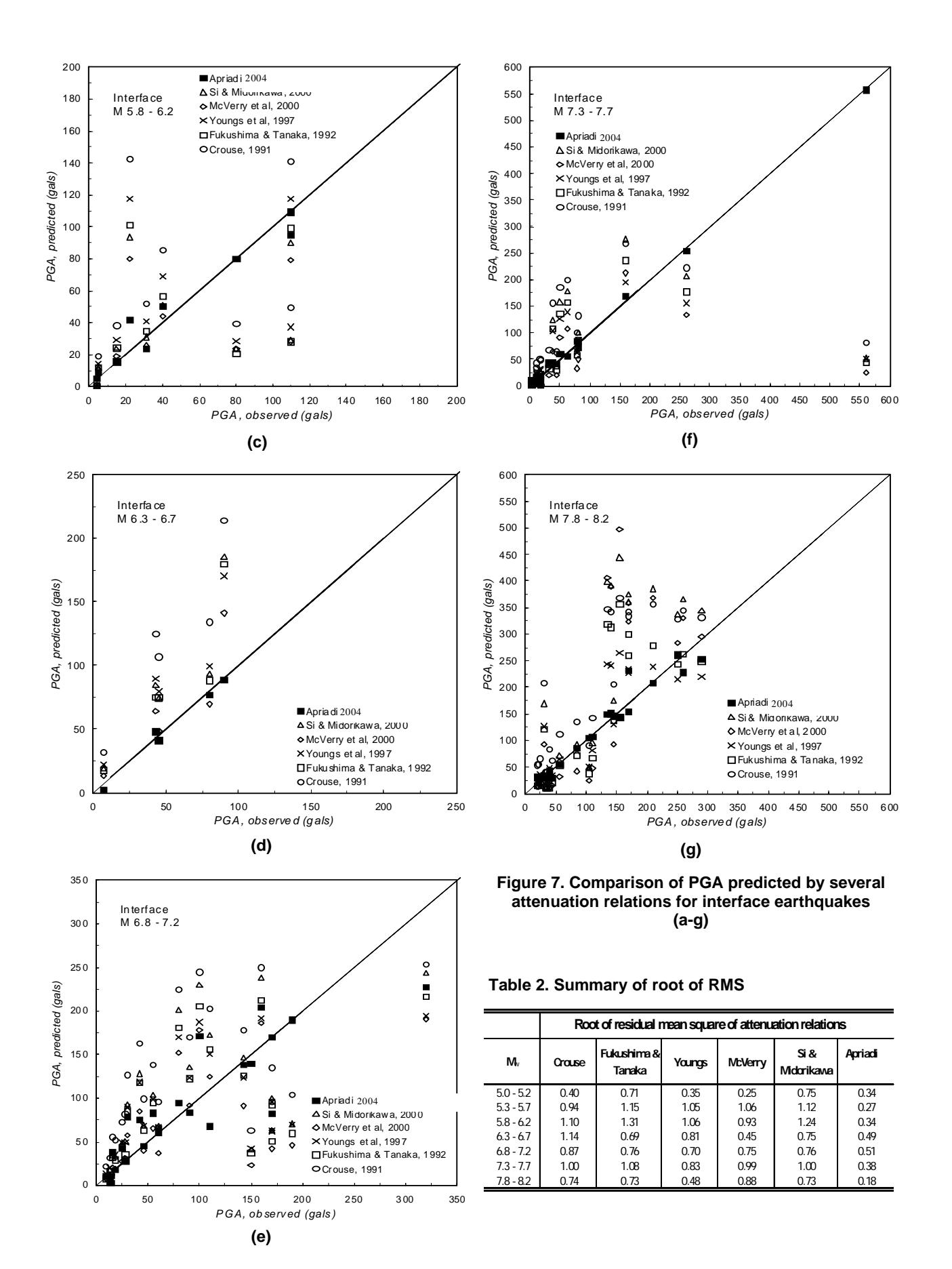
Table 3. Connection weights and % Relative Importance
| Hidden neuron (1) | H (2) | M (3) | R (3) |
|---|---|---|---|
| 1 | -0.58 | -0.35 | 4.16 |
| 2 | 0.45 | -1.63 | 0.40 |
| 3 | -0.76 | 0.84 | -1.70 |
| 4 | 1.05 | -0.73 | 8.19 |
| % RI | 15.8 | 17.8 | 66.4 |
They indicate that the ANN-based attenuation relation predictions are more consistent than the other.
4.4 Interpreting connection weights
Parameters study of the various input factors from the attenuation relations could be assessed by examining the input-hidden-output connection weights. This is carried out by partitioning the hidden-output node weights into components connected with each input node weights [Garson, 1991]. Table 3 shows the weights of the input-hidden and hidden-output layer connections and also percentage of Relative Important for the ANN-based attenuation relation.
The results show that the most important input factor for the attenuation relations are the earthquakes distance (R) is about 66.4%, Magnitude (M) is about 17.8 %, and Focal Depth (H) is about 15.8%, respectively.
5. Conclusions and Recommendations
An ANN-based attenuation relation was employed to predict strong ground motion of subduction zone earthquakes. The results show that the proposed attenuation relation is reliable and accurate to predict peak ground acceleration (PGA) due to earthquakes. In the next study, we would like to develop ANNbased attenuation relation for the strike-slip earthquakes and implement this attenuation relation to the EQRISK computer program for seismic hazard analysis.
6. Acknowledgments
Special thanks to my wife Irma for her support in this research and to prepare this paper and also to my colleagues at Geotechnical Engineering Laboratory ITB.