
Abstrak
Pada studi ini diteliti metode untuk menggabungkan metode elemen hingga (FEM) dengan metode elemen batas (BEM) dalam menyelesaikan masalah-masalah analisis struktur. Fokus penelitian adalah mengembangkan dan memilih metode yang praktis untuk menggabungkan sistem persamaan linier yang diturunkan dari FEM dan BEM menjadi satu sistem persamaan global, dan untuk mempelajari efisiensi dan akurasi dari metode gabungan. Metode penggabungan yang diterapkan pada dasarnya mentransformasikan sistem persamaan BEM menjadi bentuk yang dapat dirakit ke sistem persamaan global FEM. Sistem gabungan dipergunakan untuk menyelesaikan masalah analisis struktur gedung dengan sistem struktur portal dan dinding geser. Dinding geser dimodelkan dengan BEM plane stress, sedangkan portal dimodelkan dengan FEM balok-kolom. Metode gabungan diterapkan menjadi program komputer. Akurasi dan efisiensi metode gabungan dipelajari dengan menyelesaikan analisis struktur gedung 8 lantai dengan sistem portal-dinding geser. Sistem gabungan lebih rumit dalam proses pemrogramannya, tetapi keuntungan diperoleh dari kemudahan pembuatan model struktur dan peningkatan efisiensi dalam pemakaian memori komputer dan waktu penyelesaian.
Kata-kata Kunci: Boundary element, finite element, penggabungan, analisis struktur, dinding geser, portal.
1. Introduction
The FEM is the most popular method for structural analysis by computer. One of the most attractive features of the FEM is that the system of linear equations generated by the method has advantageous properties such as sparse, often symmetric and positive definite.
On the other hand the BEM is not as popular despite its potential advantages resulted from reducing the spatial order of element by one level. Compared to the FEM, the main advantages of the BEM are reduced complexity in domain discretization, and increased accuracy compared to the FEM with the same number of degree of freedom (DOF).
For structural analysis of shear wall-frame building, the FEM is the most suitable for modeling the frames. However the FEM may not be the best method for modeling the shear walls. Parasitic shear phenomena, for example, reduce the accuracy of low order FEM since the FEM model is too stiff in bending except if a very fine mesh is used (Kwan, 1993; Alyavuz, 2007). The source of the problem is the inability of the elements to deform following the curved deformation of bending mode. Since the shear wall resist load mostly in bending mode, this can be a serious problem. The BEM can be very competitive for modeling shear wall structure. Beside reduced complexities in domain discretization, another strong point of using the BEM is that with suitable element choice, for example a quadratic BEM, the parasitic shear phenomena can be removed from the model.
In this research, a coupled FEM-BEM method where the frames are modeled by beam-column FEM, while the shear walls are modeled by quadratic plane stress BEM is proposed. Implementation of the FEM and the BEM for solving a structural problem requires coupling method to combine system of equations from the FEM and the BEM into a global system of equations. Coupling the two systems of linear equations, derived from the FEM and the BEM that are not compatible is the main challenge of this study.
2. Linear Elastostatic Governing Equations
The governing differential equation of equilibrium for element of an isotropic linear elastic body can be written as:
\[\begin{split} &\frac{\partial \sigma_{11}}{\partial x_1} + \frac{\partial \sigma_{12}}{\partial x_2} + \frac{\partial \sigma_{13}}{\partial x_3} + f_1 = 0 \\ &\frac{\partial \sigma_{21}}{\partial x_1} + \frac{\partial \sigma_{22}}{\partial x_2} + \frac{\partial \sigma_{23}}{\partial x_3} + f_2 = 0 \\ &\frac{\partial \sigma_{31}}{\partial x_1} + \frac{\partial \sigma_{32}}{\partial x_2} + \frac{\partial \sigma_{33}}{\partial x_3} + f_3 = 0 \end{split} \tag{1}\] or using indicial notation as
\[\frac{\partial \sigma_{ij}}{\partial x_i} + f_i = 0 \quad \text{or } \sigma_{ij,j} + f_i = 0\] (2)
where \(\sigma_{ij}\) are the stress components and \(f_i\) the components of body forces per unit volume. Stress and strain components in a linear isotropic elastic solid are related by Hooke's law as follows
\[\sigma_{ij} = \lambda \delta_{ij} \epsilon_{kk} + 2\mu \epsilon_{ij} \tag{3}\] where \(\lambda\) and \(\mu\) are Lame parameters and \(\delta_{ij}\) is the Kronecker delta.
The strains and displacements are related by
\[\varepsilon_{ij} = \frac{1}{2} \left( \frac{\partial u_i}{\partial x_j} + \frac{\partial u_j}{\partial x_i} \right) = \frac{1}{2} \left( u_{i,j} + u_{j,i} \right)\](4)
The governing differential equation is subject to boundary conditions. For example, over a part of the boundary S displacement are assumed to be known (termed essential boundary condition).
\[u_k = \overline{u}_k \text{ on } \Gamma_1\] (5)
while over the remaining part of S the surface traction are prescribed (termed as traction boundary condition)
\[t_k = \sigma_{ii} n_i = \bar{t}_k \text{ on } \Gamma_2\] (6)
where \(\,\overline{\boldsymbol{u}}_{\,k}\,\) and \(\,\overline{\boldsymbol{t}}_{\,k}\,\) are the specified conditions on the boundary.
3. The FEM Formulation
The following is the FEM formulation summarized from (Bathe, 1996; Beer, 1992; Hughes, 1987). In the FEM method, the governing differential equation is transformed into its weak form by multiplying with weight function (w) that satisfy the essential boundary condition and performing integration by part
\[\int_{\Omega} \left( \sigma_{kj,j} + f_k \right) w_k d\Omega = 0 \tag{7}\]
\[-\int_{\Omega} \sigma_{kj} \varepsilon_{kj}^* d\Omega + \int_{\Omega} f_k w_k d\Omega = -\int_{\Gamma} w_k T_k d\Gamma\] (8)
With introduction of interpolation functions such that
\[\mathbf{u}_{k} = \sum_{i=1}^{\text{made}} \mathbf{N}_{i} \mathbf{u}_{ki}\] Equation (8) can be transformed into element
response matrices. Contributions of all element matrices are assembled to get the matrix equation that represents the response matrix of the problem domain:
\[\mathbf{K} \mathbf{u} = \int_{\Omega} \mathbf{N}^{\mathrm{T}} \mathbf{f}_{k} d\Omega + \int_{\Gamma} \mathbf{N}^{\mathrm{T}} \mathbf{t}_{k} d\Gamma\] (9)
\[[\mathbf{K}]\{\mathbf{u}\} = \{\mathbf{f}\}\tag{10}\] where, K is termed stiffness matrix, u is displacement vector and f is force vector. The force vector f is formed from two components that is body forces and
\[\{\mathbf{f}\}_{\text{body foce}} = \int_{\Omega} \mathbf{N}^{\mathsf{T}} \mathbf{f}_{k} d\Omega\] \[\{\mathbf{f}\}_{\text{traction}} = \int_{\Gamma} \mathbf{N}^{\mathsf{T}} \mathbf{t}_{k} d\Gamma\] (11)
4. The BEM Formulation
The following is the BEM formulation summarized from (Banerjee, 1994; Beer, 1992; Beskos, 1984; Zafrany, 1993).
The basics equation for the BEM is achieved by performing integration by part to Equation (8) to get:
\[-\int_{\Omega} \sigma_{kj,j}^* u_k d\Omega + \int_{\Omega} f_k u_k^* d\Omega = -\int_{\Gamma} u_k^* T_k d\Gamma + \int_{\Gamma} u_k T_k^* d\Gamma\] (12)
The weighting function in the BEM is the solution of a basic elastic problem corresponding to an infinite domain loaded with a concentrated unit point load. This solution is known as fundamental solution. The application of the fundamental solution to Equation (12) resulted in Somigliana's identity that gives the value of displacements at any internal point in terms of the boundary value of displacements and tractions, the body forces and known fundamental solution:
\[u_1^i + \int_{\Gamma} u_k T_k^* d\Gamma = \int_{\Gamma} u_k^* T_k d\Gamma + \int_{\Omega} f_k u_k^* d\Omega\] (13)
Integral equations on a boundary node are formed by assuming a node i is on the boundary, but its domain is represented by hemisphere with radius e for 3D or ½ circle for 2D. Node x<sup>1</sup> is at the centre. As the radius e decreased to zero, the node then become a boundary node and Equation (13) take a special form:
\[c_{lk}^{i}u_{k}^{i} + \int_{\Gamma} u_{k}T_{k}^{*}d\Gamma = \int_{\Gamma} u_{k}^{*}T_{k}d\Gamma + \int_{\Omega} f_{k}u_{k}^{*}d\Omega\] (14)
The above equation can be written in matrix form every node i as follows:
\[\mathbf{c}^{i}\mathbf{u}^{i} + \sum_{j=1}^{N} \hat{\mathbf{H}}^{ij}\mathbf{u}^{j} = \sum_{j=1}^{N} \hat{\mathbf{G}}^{ij}\mathbf{t}^{j} + \sum_{s=1}^{M} \mathbf{B}^{is}\] (15)
where N is number of nodes, u<sup>J</sup> and t<sup>J</sup> are, respectively, displacement and traction on node j.
Combinations of all element contributions from the response coefficient matrices for the problem:
\[[\mathbf{H}]\{\mathbf{u}\} = [\mathbf{G}]\{\mathbf{t}\} + \{\mathbf{b}\} \tag{16}\] where, u and t are, respectively, displacement and traction vectors. b is contribution from body forces.
5. Coupling Theory: Combination of the FEM and the BEM
There are basically two approaches to explicitly couple FEM and BEM regions. In the first approach, the BEM region is treated as a super finite element and its stiffness matrix is computed and assembled into the global stiffness matrix of the FEM (Apicella, 1998;
Cali, 1999). In the second approach the FEM region is treated as an equivalent BEM region (Beer, 1992). Another possible method is by performing the coupling implicitly, where FEM and BEM sub-domains are analyzed separately and the coupling is enforced at their interface (Eppler, 2006; Soares, 2007). The first explicit coupling method is employed in this study and described in the following.
Consider a problem domain that is divided into BEM and FEM regions with the BEM region completely contained by the FEM region as illustrated in Figure 1. By using the BEM method, assuming no body forces, the following relation between tractions {t} and displacements {u} can be formed
\[[\mathbf{H}]\{\mathbf{u}\} = [\mathbf{G}]\{\mathbf{t}\} \tag{17}\]
since the G matrix is non-singular, it is possible to
\[\{\mathbf{t}\} = [\mathbf{G}]^{-1}[\mathbf{H}]\{\mathbf{u}\} \tag{18}\]
The nodal tractions vector in the BEM global system of equations need to be converted into nodal forces {f} so as to be consistent with FEM system of equations. This can be done by premultiplying nodal tractions by a matrix [M] derived from element shape functions.
\[\{\mathbf{f}\} = [\mathbf{M}] \{\mathbf{t}\} \tag{19}\]
Matrix [M] derived from formulation for equivalent nodal force in the FEM method. From Equation (11), equivalent nodal force fe at node j of element e due to distributed traction t is as follows
\[\mathbf{f}_{j}^{e} = \int_{Se} N_{j} \mathbf{t} dS\] (20)
with integration performed for all BEM area (S<sub>e</sub>). Traction value at any point can interpolated from traction values at element nodes
\[t = \sum_{i=1}^{\text{nnode}} N_j \mathbf{t}_j^e\] (21)
Figure 1. Problem domain divided into FEM and BEM regions
The following equations is formed by combining the two equations
\[\mathbf{f}_{i}^{e} = \sum_{j=1}^{\text{nn ode}} \left( \int_{Se} N_{i} N_{j} \, dS \right) \mathbf{t}_{j}^{e}\] (22)
Therefore the Matrix [M] is
\[\mathbf{M} = \begin{bmatrix} \mathbf{N}_{11}^{e} \mathbf{I} & \cdots & \mathbf{N}_{1j}^{e} \mathbf{I} \\ \vdots & \ddots & \vdots \\ \mathbf{N}_{ij}^{e} \mathbf{I} & \cdots & \mathbf{N}_{ij}^{e} \mathbf{I} \end{bmatrix} \quad \text{where} \quad \mathbf{N}_{ij}^{e} = \int_{S} \mathbf{N}_{i} \mathbf{N}_{j} \, d\mathbf{S}\] (23)
where I is a (2 x 2) or (3 x 3) unit matrix depending if two or three-dimensional problem is considered. The following equation is formed by substitution of Equation (18) to Equation (19)
\[\{\mathbf{f}\} = [\mathbf{M}][\mathbf{G}]^{-1}[\mathbf{H}]\{\mathbf{u}\}\] (24)
Furthermore, analogously to the FEM relation {f} = [K] FEM {u} between nodal displacement and nodal tractions, which are linked by the FEM stiffness matrix K<sub>FEM</sub>, it is possible to express:
\[[\mathbf{K}]_{\text{BEM}} = [\mathbf{M}][\mathbf{G}]^{-1}[\mathbf{H}]\] (25)
Finally the K<sub>BEM</sub> matrix for the BEM domain is assembled into the stiffness \(K_{\text{FEM}}\) matrix.
6. Partial Coupling
For structural analysis problem where not all BEM nodes interface with FEM nodes, the solution process become more complicated. Nodal traction on a FEM node may partially be given as load data while partially need to be derived from BEM system.
Consider a problem domain that is divided into BEM and FEM regions with the BEM region only partially contained by the FEM region as illustrated in Figure 2. To form a super FEM element from equations that represents the BEM region, the BEM system of equations of Equation (17) is partitioned into interface (BI) and non-interface (BN) variables. Specifically, denote the global tractions of at the interface nodes by \(\{t\}^{BI}\), the applied traction at each boundary element not at the interface by \(\{t\}^{BN}\), and the corresponding global displacement at the interface nodes by {u} and at non interface nodes by {u}BN. The partitioned BEM equation can be written as:
\[\left[\mathbf{H}^{\mathrm{BI}}, \mathbf{H}^{\mathrm{BN}}\right] \begin{Bmatrix} \mathbf{u}^{\mathrm{BI}} \\ \mathbf{u}^{\mathrm{BN}} \end{Bmatrix} = \left[\mathbf{G}^{\mathrm{BI}}, \mathbf{G}^{\mathrm{BN}}\right] \begin{Bmatrix} \mathbf{t}^{\mathrm{BI}} \\ \mathbf{t}^{\mathrm{BN}} \end{Bmatrix}\](26)
Rearrangement of Equation (26) gives
\[\left[-\mathbf{G}^{\mathrm{BI}}, \mathbf{H}^{\mathrm{BN}}\right] \begin{Bmatrix} \mathbf{t}^{\mathrm{BI}} \\ \mathbf{u}^{\mathrm{BN}} \end{Bmatrix} = \mathbf{f}^{\mathrm{BN}} - \mathbf{H}^{\mathrm{BI}} \mathbf{u}^{\mathrm{BI}}\] (27)
where \[\mathbf{f}^{BN} = \mathbf{G}^{BN} \mathbf{t}^{BN}\]
Equation (27) can be solved for \(\{t\}^{BI}\) and \(\{u\}^{BN}\)expresses in term of \(\{u\}^{BI}\):
\[\mathbf{t}^{\mathrm{BI}} = \hat{\mathbf{t}}^{\mathrm{BI}} + \mathbf{O}\mathbf{u}^{\mathrm{BI}} \quad \text{and} \quad \mathbf{u}^{\mathrm{BN}} = \hat{\mathbf{u}}^{\mathrm{BN}} + \mathbf{T}\mathbf{u}^{\mathrm{BI}}\] (28)
where \[\{\hat{\boldsymbol{t}}\}^{BI}\] and \(\{\hat{\boldsymbol{u}}\}^{BN}\)
are, respectively, nodal tractions at interface and displacements of non-interface nodes for zero displacement of the interface nodes that can be expressed as follows:
\[\begin{Bmatrix} \hat{\mathbf{t}}^{BI} \\ \hat{\mathbf{u}}^{BN} \end{Bmatrix} = \left[ -\mathbf{G}^{BI}, \mathbf{H}^{BN} \right]^{-1} \mathbf{f}^{BN}\] (29)
Note that O is solutions for the tractions at the interface nodes and T are solutions for the displacements of the non-interface nodes, both due to unit displacements of the interface nodes. Q and T symbolically can be expressed as follows:
\[\begin{bmatrix} \mathbf{Q} \\ \mathbf{T} \end{bmatrix} = \left[ -\mathbf{G}^{\mathrm{BI}}, \mathbf{H}^{\mathrm{BN}} \right]^{-1} \mathbf{H}^{\mathrm{BI}}\] (30)
To form Q and T, it is unnecessary and inefficient to form the inverse of matrix [-GBI, HBN] explicitly. Gauss elimination and triangular matrix substitutions should be used. Also note that only Q needs to be formed explicitly for inclusion into the FEM system of equations described in the followings.
The system of equations of coupled FEM and BEM can be formulated by considering traction of the interface region formulated by BEM as traction load to the FEM region. As in the full coupling, the nodal tractions vector in the BEM global system of equations need to be converted into nodal forces {f} to be consistent with FEM system of equations. This can be done by pre multiplying nodal tractions for a matrix [M] derived from element shape functions, similar to Equation (20).
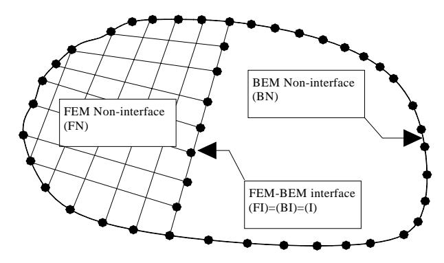
Figure 2. Problem with partial coupling of FEM and BEM regions
\[\{\mathbf{f}\}^{\mathrm{BI}} = [\mathbf{M}] \{\mathbf{f}\}^{\mathrm{BI}}\] \[= [\mathbf{M}] \{\hat{\mathbf{t}}^{\mathrm{BI}} + \mathbf{Q}\mathbf{u}^{\mathrm{BI}}\}\] \[= [\mathbf{M}] \{\hat{\mathbf{f}}\}^{\mathrm{BI}} + [\mathbf{M}] [\mathbf{Q}] \{\mathbf{u}\}^{\mathrm{BI}}\] (31)
Define: \[\hat{\mathbf{f}}^{BI} = \mathbf{M} \hat{\mathbf{t}}^{BI}\] and \(\{\mathbf{K}\}^{BI} = \frac{1}{2} [(\mathbf{MQ})^T + (\mathbf{MQ})]\)
Note that {K}<sup>BI</sup> is chosen as symmetrization of (MQ)
The FEM total system of equations including traction on BEM interface become
\[[\mathbf{K}]^{F} \{\mathbf{u}\}^{F} - \{\mathbf{f}\}^{F} + \{\mathbf{f}\}^{BI} = 0\] or \[[\mathbf{K}]^{F} \{\mathbf{u}\}^{F} - \{\mathbf{f}\}^{F} + [\mathbf{K}]^{BI} \{\mathbf{u}\}^{BI} + \{\hat{\mathbf{f}}\}^{BI} = 0\] (32)
The BEM equations are assembled into the FEM equations by using compatibility equations that ensure the displacements of the interface nodes computed by the BEM and the FEM are the same; that is \(\{u\}^{BI} = \{u\}^{FI}\)= {u}<sup>I</sup>. Therefore the global system of equations become:
\[\left[\mathbf{K}^{\mathrm{FN}}, \mathbf{K}^{\mathrm{FI}} + \mathbf{K}^{\mathrm{BI}}\right] \begin{pmatrix} \mathbf{u}^{\mathrm{FN}} \\ \mathbf{u}^{\mathrm{I}} \end{pmatrix} - \left\{\mathbf{f}\right\}^{\mathrm{F}} + \left\{\hat{\mathbf{f}}\right\}^{\mathrm{BI}} = \mathbf{0}\] (33)
Solution of Equation (33) gives the displacements at the interface and inside the FEM region. To obtain the displacements at the non-interface nodes and tractions at interface nodes, substitute the displacements at the interface into Equation (28).
7. Constraint for Rotation-Displacement Compatibility
For frame and shear wall structure where the frame members are modeled by beam-columns FEM model while the shear wall is modeled as plane stress FEM or BEM, interface of the two element types require careful consideration. To ensure compatibility between beam column element that has rotational and translation DOFs to plane stress element that has only translation DOFs, interface elements are employed. The interface elements are beam-columns elements that are perpendicular to the real beam-column element with joint displacement constrained to model the condition where any cross section of the beam-column perpendicular to its axis remains plane. The interface element is shown in Figure 3.
The constraint equations can be written as follows:
8. Summary of Solution Procedure
The solution procedure can be summarized as follows
1. Restraint interface nodes and apply load on noninterface nodes.
\[\{\mathbf{u}\}^{\mathrm{B}} = \{0\}, \text{ and}\] \[\{\mathbf{t}\}^{\mathrm{B}} = \{\hat{\mathbf{t}}\}^{\mathrm{B}} + \hat{\mathbf{Q}}\{\mathbf{u}\}^{\mathrm{B}} = \{\hat{\mathbf{t}}\}^{\mathrm{B}}\] \[\{\mathbf{u}\}^{\mathrm{C}} = \{\hat{\mathbf{u}}\}^{\mathrm{C}} + \mathbf{G}\{\mathbf{u}\}^{\mathrm{B}} = \{\hat{\mathbf{u}}\}^{\mathrm{C}}\] Solve \[\{\hat{\mathbf{t}}\}^{\mathrm{BI}} \text{ and } \{\hat{\mathbf{u}}\}^{\mathrm{BN}} \text{ using}\] \[\{\hat{\mathbf{t}}\}^{\mathrm{BI}} = [-\mathbf{G}^{\mathrm{BI}}, \mathbf{H}^{\mathrm{BN}}]^{-1} \mathbf{f}^{\mathrm{BN}}\]
2. Remove loads and apply unit displacements to interface nodes
\[\{\mathbf{u}\}_{1}^{\mathrm{BI}} = \begin{cases} 1\\0\\...\\0 \end{cases} , \{\mathbf{u}\}_{2}^{\mathrm{BI}} = \begin{cases} 0\\1\\0\\...\\0 \end{cases} ; .... \{\mathbf{u}\}_{n}^{\mathrm{BI}} = \begin{cases} 0\\...\\1 \end{cases}\]
Figure 3. Interface Element where n is the number of interface nodes
Solve the following system of equations for each interface node i = 1... n
\[\left[ -\mathbf{G}^{\mathrm{BI}},\,\mathbf{H}^{\mathrm{BN}} \right] \left\{ \begin{matrix} \mathbf{t}^{\mathrm{BI}} \\ \mathbf{u}^{\mathrm{BN}} \end{matrix} \right\} = \left\{ \mathbf{f} \right\}^{\mathrm{BN}} - \left[ \mathbf{H} \right]^{\mathrm{BI}} \, \left\{ \mathbf{u} \right\}^{\mathrm{BI}}_{\mathrm{i}}\]
From the relations:
\[\begin{split} &\left\{\boldsymbol{t}\right\}^{BI} = \left\{\boldsymbol{\hat{t}}\right\}^{BI} + \left[\boldsymbol{Q}\right] \left\{\boldsymbol{u}\right\}^{BI}_{i} = \left\{\boldsymbol{\hat{t}}\right\}^{BI} + \left[\boldsymbol{Q}\right]_{i} \text{ , and} \\ &\left\{\boldsymbol{u}\right\}^{BN} = \left\{\boldsymbol{\hat{u}}\right\}^{BN} + \left[\boldsymbol{T}\right] \left\{\boldsymbol{u}\right\}^{BI}_{i} = \left\{\boldsymbol{\hat{u}}\right\}^{BN} + \left[\boldsymbol{T}\right]_{i} \end{split}\]
The following relations can be formed for each
\[\left[\mathbf{Q}\right]_{i}=\left\{\mathbf{t}\right\}^{BI}-\left\{\hat{\mathbf{t}}\right\}^{BI}\] and
\[\left[\mathbf{T}\right]_{i} = \left\{\mathbf{u}\right\}^{\mathrm{BN}} - \left\{\hat{\mathbf{u}}\right\}^{\mathrm{BN}}\]
Form Q and T by collecting vectors fomed above
\[[\mathbf{Q}] = [\mathbf{Q}_1; \mathbf{Q}_2; \cdots; \mathbf{Q}_n]\]\[[\mathbf{T}] = [\mathbf{T}_1; \mathbf{T}_2; \cdots; \mathbf{T}_n]\]
3. Form \[\hat{\mathbf{f}}^{BI} = \mathbf{M} \hat{\mathbf{t}}^{BI}\] and \(\{\mathbf{K}\}^{BI} = \frac{1}{2} [(\mathbf{MQ})^T + (\mathbf{MQ})]\)
4. Form and solve global FEM system
\[\left[\mathbf{K}^{\mathrm{FN}}, \mathbf{K}^{\mathrm{H}} + \mathbf{K}^{\mathrm{BI}}\right] \left\{ \mathbf{u}^{\mathrm{FN}}_{\mathbf{u}^{\mathrm{I}}} \right\} = \left\{ \mathbf{f} \right\}^{\mathrm{F}} - \left\{ \hat{\mathbf{f}} \right\}^{\mathrm{BI}}\]
5. Substitute to get BEM solution:
\[\mathbf{t}^{\mathrm{BI}} = \hat{\mathbf{t}}^{\mathrm{BI}} + \mathbf{O}\mathbf{u}^{\mathrm{BI}} \text{ and } \mathbf{u}^{\mathrm{BN}} = \hat{\mathbf{u}}^{\mathrm{BN}} + \mathbf{T}\mathbf{u}^{\mathrm{BI}}\]
9. Numerical Example
The coupling method presented in this above has been implemented on a personal computer. For the purpose of examining the accuracy and efficiency of the coupled BEM-FEM method, a shear wall-frame building structure problem as shown in Figure 4 is solved by the both FEM and coupled BEM-FEM methods. Elements sizes in the example problem are: shear wall thickness = 30 cm, beams = \(30 \text{ x } 40 \text{ cm}^2\) and columns = 40 x 40 cm<sup>2</sup>. For accuracy comparison, the analysis with FEM model is performed with three levels of mesh refinement (Model A, Model B and Model C). The models for the FEM and the coupled FEM-BEM are shown in Figure 5.
Features of the model for the coupled FEM-BEM method are:
- 1. Shear wall is modeled by 152 two dimensional BEM quadratic elements.
- 2. Each beam and column modeled by one beam column FEM model.
- 3. The rotational degree of freedom of the FEM is transformed to the BEM by a constraint model.
Figure 4. Shear wall-frame building
Features of the model for the coupled FEM-BEM method are:
- 1. Shear wall is modeled by membrane-shell FEM quadrilateral model. The number of element used for model A, B and C are, respectively, (4x16), (10x80) and (20x160).
- 2. Each beam and column modeled by one segment beam column FEM model.
The number of nodes, elements and degree of freedom (DOF) for the models are compared in Table 1. Note from the table that the number of DOF of the coupled method model is less than half of the number of DOF for Model B.
The results of the analysis for all models are compared in Figure 6, Figure 7, Table 2 and Table 3. Figure 6 shows comparisons of vertical and horizontal displacements as predicted by the models. Horizontal displacement values and relative error with respect to Model C are presented in Table 2. The figure and table show that using the FEM with coarse model (Model A) resulted in significant underestimate of both vertical and horizontal displacements. The figures also show that the results of coupled FEM-BEM are very close to results of the FEM model with very fine mesh (Model
Figure 7 shows comparisons of shear wall moment distribution as predicted by FEM with very fine mesh (Model C) and by coupled FEM-BEM model. The figure shows that the shear wall moment distribution predicted by coupled FEM-BEM can match the accuracy of the FEM model with very fine mesh (Model C).
Comparison of shear wall moment distribution of FEM Model C with FEM-BEM model is shown in Figure 7 and Table 3 compare ground level shear wall moments predicted using the four models. The relative error shown in column three of the table is computed with respect to results from Model C (assuming results from Model C as the exact values). The table shows that the accuracy of the coupled FEM -BEM model in terms of ground level shear wall moment is much better that the accuracy of Model A. Only very small differences are observed between results of the FEM-BEM model and the FEM model with very fine mesh (Model A).
Table 1. Comparison of number of problem variables (for each story)
| Element | Number of | |||||
|---|---|---|---|---|---|---|
| MODEL | Model | Element | Node | DOF | ||
| Model A | BC | 4 | 4 | 12 | ||
| SW | 4 | 15 | 45 | |||
| Model B | BC | 4 | 4 | 12 | ||
| F | SW | 100 | 121 | 363 | ||
| E | BC | 4 | 4 | 12 | ||
| M | Model C | SW | 400 | 441 | 1323 | |
| Coupled FEM-BEM | BC | 4 | 4 | 12 | ||
Note: BC = beam-column; SW = shear wall
Table 2. Comparison of horizontal displacements
| Model A | Model B | Model C | Coupled FEM-BEM | ||||
|---|---|---|---|---|---|---|---|
| Story | Value | Error(%) | Value | Error(%) | Value | Value | Error(%) |
| 0 | 0.000 | 0.0 | 0.000 | 0.0 | 0.000 | 0.000 | 0.0 |
| 1 | 0.011 | 15.6 | 0.012 | 4.4 | 0.013 | 0.012 | 3.7 |
| 2 | 0.036 | 13.6 | 0.040 | 4.8 | 0.042 | 0.042 | 0.0 |
| 3 | 0.072 | 13.6 | 0.079 | 5.1 | 0.083 | 0.084 | 0.7 |
| 4 | 0.114 | 14.0 | 0.126 | 5.4 | 0.133 | 0.134 | 1.0 |
| 5 | 0.160 | 14.5 | 0.176 | 5.7 | 0.187 | 0.189 | 1.0 |
| 6 | 0.207 | 14.9 | 0.228 | 6.0 | 0.243 | 0.245 | 0.6 |
| 7 | 0.254 | 15.3 | 0.281 | 6.3 | 0.300 | 0.303 | 1.0 |
| 8 | 0.300 | 15.7 | 0.333 | 6.5 | 0.356 | 0.362 | 1.5 |
Table 3. Comparison of ground level shear wall moments
| MODEL | Moment | Relative Error |
|---|---|---|
| Model A | 51529 | 12.3 % |
| Model B | 57275 | 2.5 % |
| Model C | 58740 | - |
| Coupled FEM-BEM | 57493 | 2.1% |
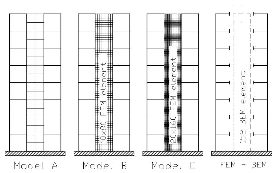
Figure 5. FEM models with various mesh refinement (Model A, B and C) and the coupled FEM-BEM model

Figure 6. Comparison of horizontal and vertical displacements
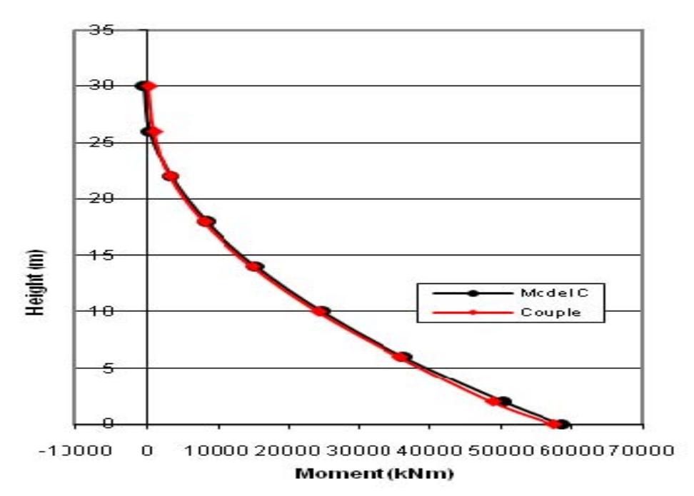
Figure 7. Comparison of shear wall moments
10. Conclusions
- 1. The FEM and the BEM have advantages and disadvantages compared to each other, and the advantages of both methods can be exploited if the FEM and the BEM are coupled. The coupled FEM and BEM method has been successfully implemented into a computer program. With the coupled method, a problem domain can be separated into regions so that the FEM or the BEM can be used to model regions that are most suitable for each method. The system of equations from the FEM and BEM are combined into a single global system of equations.
- 2. The coupled FEM and BEM method has been implemented successfully for structural analysis of shear wall-frame building where shear walls and frames are modeled, respectively, by the BEM and the FEM. It can be concluded that the coupled method is much more complicated to implement compared to the FEM. However, the couple method has advantages in term of reduced complexity in mesh generation and increased efficiency in both memory requirement and computing time. From numerical experiments it is found that for equal level of accuracy the coupled method requires much lower degree of freedoms compared to the FEM.