
Abstrak
Penelitian ini dimaksudkan untuk mencari hubungan antara tingkat kekritisan umur waduk dengan inflow sedimen. Tingkat kekritisan umur waduk didefinisikan sebagai perbandingan antara umur rencana waduk dengan umur efektifnya. Umur efektif waduk dipengaruhi oleh jumlah sedimen yang masuk ke waduk serta efisiensi pengendapan sedimen. Model Soil and Water Assessment Tool (SWAT) versi 2005 digunakan dalam penelitian ini untuk mensimulasikan proses-proses hidrologi yang terjadi di daerah tangkapan. Keandalan model SWAT sangat bergantung pada ketersediaan data dan penyesuaian beberapa parameter. Dari hasil kalibrasi dan validasi terhadap data bulanan, kinerja model dinilai cukup baik. Hasil simulasi menunjukkan bahwa sediment yield rata-rata sebesar 235,86 ton/ha/tahun, serta inflow sedimen rata-rata yang masuk ke waduk sebesar 5.102.000 ton per tahun yang ekivalen dengan 3.836.090 m3 per tahun yang menghasilkan umur waduk sebesar 43,66 tahun (21,66 sisa umur waduk) yang bersesuaian dengan tingkat kekritisan 2,29. Grafik yang menghubungan nilai inflow sedimen dengan tingkat kekritisan umur waduk menunjukkan hubungan yang bersifat linear.
Kata-kata Kunci: Kapasitas waduk, umur waduk, inflow tahunan, efisiensi pengendapan sedimen.
1. Introduction
The Saguling reservoir catchment covers the fountain of the Citarum river down to Saguling with an area of 1744.98 km<sup>2</sup> as a part of the Citarum watershed, one of the biggest watershed in West Java. The average observed monthly rainfall in 2008 is about 172 mm with the total annual rainfall of 2,070 mm. The topography of the region is dominated by mountains along the borders and a broad plain in the middle. The sedimentation rate in the Upper Citarum watershed in the last decade is reported to be increasing. It is indicated by the mean sedimentation rate of 4.048.132 ton per year (PT Indonesia Power, 2008). The fact is due to the ecosystem degradation and the decreasing forest area over the watershed and the catchment of the Saguling reservoir. The aim of this study is to analyse the effect of the sediment inflow on the critical degree of reservoir lifetime for the Saguling reservoir (Poerbandono, 2006).
2. Methods
Erosion is the lifting up of soil layer or sediment due to the tractive stresses which is generated by the movement of wind or water on the soil surface or channel. In the watershed environment the erosion rate is controlled by the velocity of the flowing water and the sediment properties (mainly the grain size). The tractive stresses working on the soil surface or channel are equivalent to the velocity of the flow. The resistance of the soil or sediment to the movement is equivalent to its grain size. The external driving forces that cause erosion to occur are rainfall and flowing water on the slopes of the watershed. The high rainfall and steep slopes are the main factors that lead to erosion. The resistance of the catchment to erosion depends chiefly on the land cover. The resistance reinforcement to erosion can also be achieved through engineering measures. In this study the erosion and sedimentation behaviour is modeled using ArcSWAT tool (Arc GIS Interface for SWAT Model). SWAT model (Soil and Water Assessment Tool) is a semidistributed watershed model with ArcGIS interface delineating subbasins and river networks from digital elevation model and calculating the daily water balance from meteorological, soil and land use data.
The erosion modeling in SWAT is based on the following Modified Universal Soil Loss Equation (MUSLE) equation (Neitsch, 2005):
\[sed=1\,1\,8\cdot\left(Q_{surf}\cdot Q_{peak}\cdot areq_{vu}\right)^{0.56}\cdot K_{USLE}\cdot C_{USLE}\cdot P_{USLE}\cdot LS_{USLE}\cdot CFRC\] where:
= sediment yield (ton) sed = surface runoff (mm/ha) \(Q_{surf}\)= peak runoff rate \((m^3/s)\)\(Q_{peak}\)
= area of the HRU (hydrologic response \(area_{hru}\)unit (ha)
\(K_{USLE}\)= USLE soil erodibility factor (0.013 ton
\(m^2 hr/[m^3 ton cm]\)\(C_{USLE}\)= USLE cover and management factor
\(P_{\mathit{USLE}}\)= USLE support practice factor \(LS_{USLE}\)USLE topographic factor
CFRGcoarse fragment factor
3. Effective Lifetime of A Reservoir
The effective lifetime of a reservoir is estimated using tap efficiency method. Gunner Brune (Bureau of Reclamation, 2006) found that the tap efficiency depends on the ratio between the reservoir capacity (C) and annual inflow \((I_w)\). Tap efficiency will be decreasing over the lifetime of the reservoir due to the reduction in its capacity by the accumulated sediment. Equation 1 is used to determine the tap efficiency:
where:
sed = sediment yield (ton)
surface runoff (mm/ha) Qsurf
\(Q_{peak}\)= peak runoff rate \((m^3/s)\)
\(area_{hru}\)area of the HRU (hydrologic response
unit (ha)
\(K_{USLE}\)= USLE soil erodibility factor (0.013 ton
\(m^2 hr/[m^3 ton cm]\)
\(C_{USLE}\)= USLE cover and management factor
\(P_{USLE}\)= USLE support practice factor \(LS_{USLE}\)= USLE topographic factor CFRG = coarse fragment factor
\[TE = 0.96^{0.25 \log C / I_W}\] (1)
where:
TE= tap efficiency (%)
C= reservoir effective capacity (m<sup>3</sup>)
= mean annual inflow \((m^3)\)\(I_w\)
The volume of the reservoir dead storage after t years can subsequently be calculated as:
\[DEAD_{t=n} = \int_{1}^{n} \frac{sed_{out}}{\gamma_{sed}} \cdot TE(t) \cdot dt\] (2)
where:
\(DEAD_{t=n}\) = dead storage volume after n years (m<sup>3</sup>)
= number of taken years into consideration
= tap efficiency as a function of time TE(t)
= sediment inflow, the amount of sediment \(sed_{out}\)flowing out of the catchment and entering the reservoir, which is one of the SWAT outputs (ton/year)
\(g_{sed}\)specific gravity of the sediment (ton/m<sup>3</sup>)
Substituting Equation 1 into Equation 2, we obtain:
\[DEAD_{t=n} = \frac{sed_{out}}{\gamma_{sed}} \cdot \int_{1}^{t} 0.96^{0.25 \log \left(\frac{C(t)}{I_{w}}\right)} \cdot dt\] (3)
where:
C(t) =reservoir effective capacity as a function of
Considering, \(C(t) = C_a - DEAD_{t-1}\) hence:
\[DEAD_{t=n} = \frac{sed_{out}}{\gamma_{sed}} \cdot \int_{1}^{t} 0.96^{0.25 \log \left(\frac{C_o - DEAD_{t-1}}{I_w}\right)} \cdot dt\] (4)
where:
\(C_o\)= reservoir total capacity (m<sup>3</sup>) \(DEAD_{t-1}\) = dead storage volume in the preceding
The above equation will be too complicated to solve analytically. Alternatively, we can rewrite it into a discrete form:
\[DEAD_{t=n} = \frac{sed_{out}}{\gamma_{sed}} \cdot \sum_{t=1}^{t=n} 0.96^{0.25 \log \left(\frac{C_o - DEAD_{t-1}}{I_w}\right)} \cdot \Delta t\] (5)
or:
\[DEAD_{t=n} = \frac{sed_{out}}{\gamma_{sed}} \cdot \Delta t \cdot \sum_{t=1}^{n} 0.96^{0.25 \log \left(\frac{C_o - DEAD_{t-1}}{I_w}\right)}\] (6)
where:
Dt = time step (year)
The Equation 6 above can be solved numerically:
1. for dead storage design purpose, the value of \(DEAD_{t=n}\) can be determined directly by setting n equal to the designated lifetime of the reservoir \((U_r)\), 2. whereas for obtaining the effective lifetime of the reservoir \((U_e)\) which is represented by n, the value of n can be determined indirectly by setting \(DEAD_{t=n}\) equal to the total volume of the dead storage.
4. Critical Degree of Reservoir Lifetime
In this study the critical degree of a reservoir is considered upon its functionality in which a reservoir is considered to be critical when its effective lifetime is equal to its designated lifetime. The effective lifetime of a reservoir is the period required for the sediment to fill the dead storage full capacity, which can be higher or lower than its designated lifetime. The effective lifetime of the reservoir is obtained indirectly using Equation 6 previously mentioned. In general, the critical degree of reservoir lifetime can be defined as:
\[c = \frac{U_r}{U_e} \tag{7}\] where:
c = critical degree of reservoir lifetime,
\(U_e\) = reservoir effective lifetime obtained indirectly from Equation 6,
\(U_r = reservoir designated lifetime.\)
The critical condition is achieved when \(U_e = U_r\) or:
\[c = \frac{U_r}{U_r} = 1 \tag{8}\]
Thus, a reservoir will be in a critical condition when \(c \ge 1\). The critical degree of reservoir lifetime is schematically illustrated in Figure 1.
5. Model Setup Using ArcSWAT
The input data for the model setup originate from various sources (see Table 1).
Climate data was obtained from the eight weather stations spreading over the the upper Citarum watershed. The locations of the stations are listed in Table 2.
The daily rainfall from 1987 to 2008 was obtained from the eight weather stations located in the watershed. The daily rainfall so obtained is consecutively processed using pcpSTAT program to extract statistical parameters needed for the SWAT model input.
After preparing all input datasets and adding them into the SWAT user databases, a new SWAT project was created with the ArcGIS User Interface. The main steps of the procedure included delineating subbasins and HRUs and writing all input files.
Figure 1. Schematic concept of the critical degree of reservoir lifetime (modified from Morris & Fan, 1997)
Table 1. Model input data and corresponding data sources
| Type of Data | Scale | Source | Description | ||
|---|---|---|---|---|---|
| Digital elevation model | 90 m resolution | Shuttle Radar Topographic | Elevation, length and slope | ||
| Projection: UTM/WGS84 | Mission (SRTM) | ||||
| zone 48 S | |||||
| River networks (hydrography) | 1:250.000 | West Java Water Resources | |||
| Projection: UTM/WGS84 | Agency | ||||
| zone 48 S | |||||
| Geology | 1:250.000 | Soil and Agro climate Re | Soil physical properties (bulk | ||
| Projection: UTM/WGS84 | search Centre | density, texture, organic matter, | |||
| zone 48 S | hydraulic conductivity, etc.) | ||||
| Landuse/ | 1:250.000 | West Java Spatial Planning | Landuse classification | ||
| Landcover | Projection:UTM/WGS84 | Agency | |||
| zone 48 S | |||||
| Rainfall | 8 stations | Saguling reservoir authority | |||
| 1987-2004 | |||||
| Streamflow and sediment | 1 station | Saguling reservoir authority | |||
| 1987-2004 | |||||
Source: from various sources
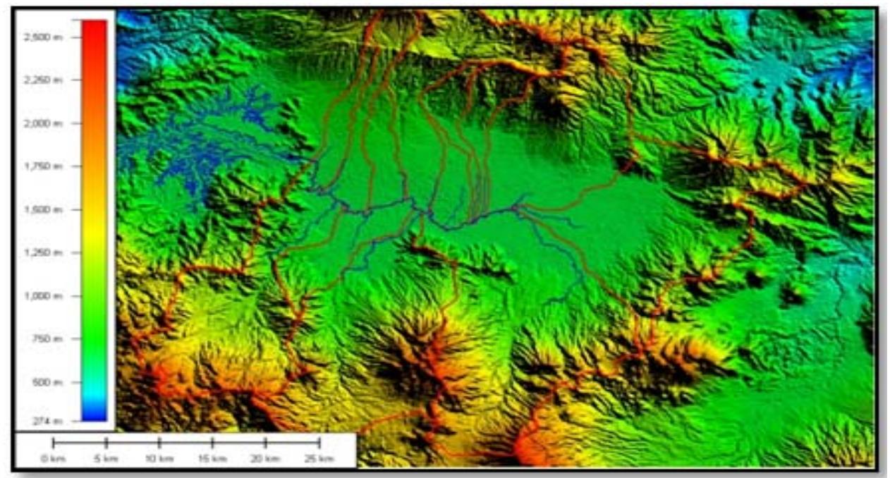
Figure 2. Digital elevation model of the upper Citarum watershed
Table 2. Locations of weather stations in the upper Citarum watershed
| No. | Station | Xpr | Ypr | Lat | Long | Elevation | |
|---|---|---|---|---|---|---|---|
| 1 | Bandung | 788962.199 | 9235110.381 | -6.913 | 107.615 | 946 | |
| 2 | Ujungberung | 797444.988 | 9234628.404 | -6.917 | 107.692 | 680 | |
| 3 | Cicalengka | 810651.148 | 9226627.592 | -6.988 | 107.811 | 673 | |
| 4 | Ciparay | 798601.732 | 9220747.477 | -7.042 | 107.703 | 689 | |
| 5 | Paseh | 803999.871 | 9213517.827 | -7.107 | 107.752 | 878 | |
| 6 | Cililin | 772285.807 | 9230387.010 | -6.956 | 107.464 | 686 | |
| 7 | Cisondari | 779804.643 | 9213421.432 | -7.109 | 107.533 | 1150 | |
| 8 | Chinchona | 785973.944 | 9206673.759 | -7.170 | 107.589 | 1458 | |
Source: West Java Water Resources Agency
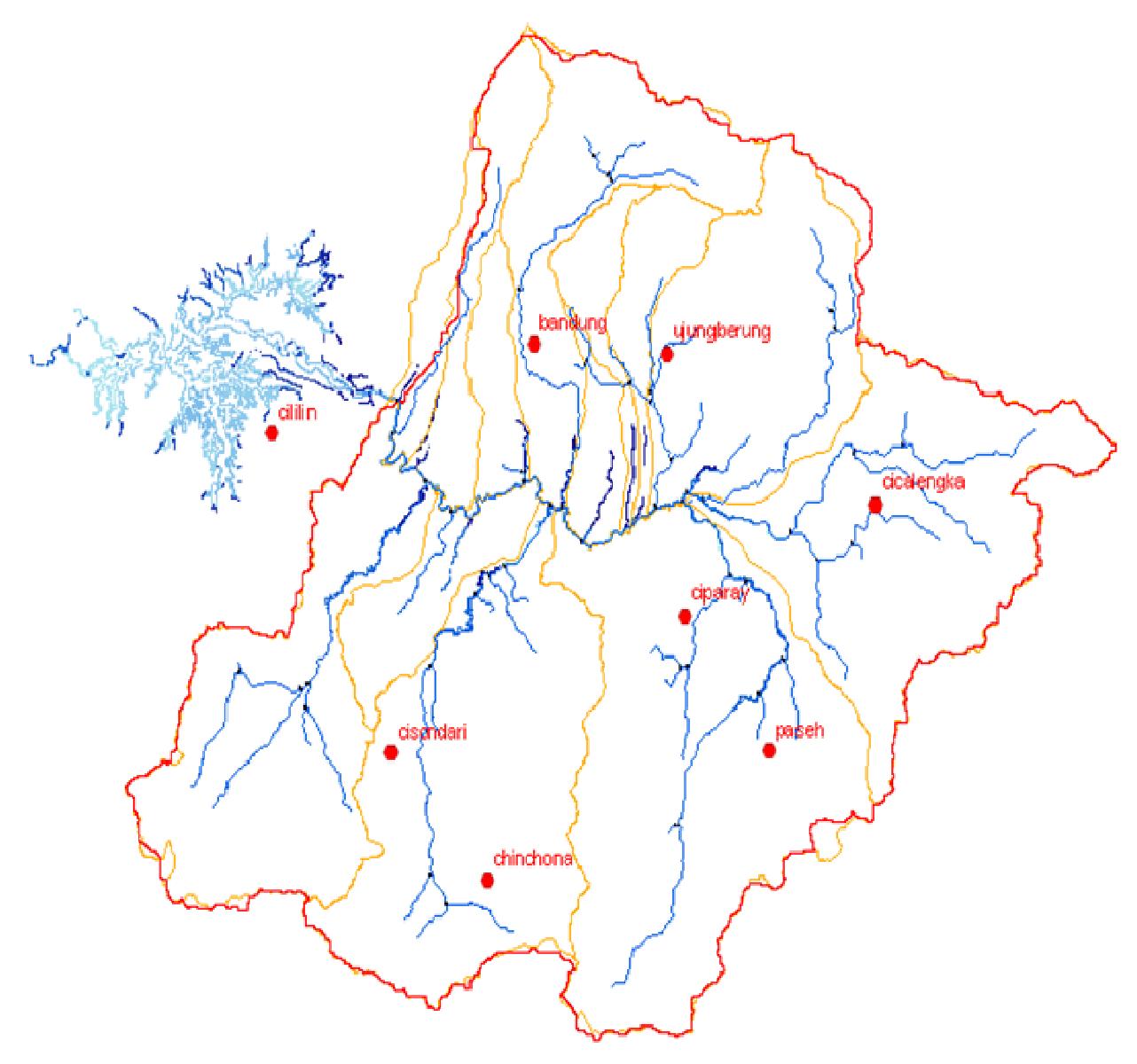
Figure 3. Locations of weather stations Source: Analysis
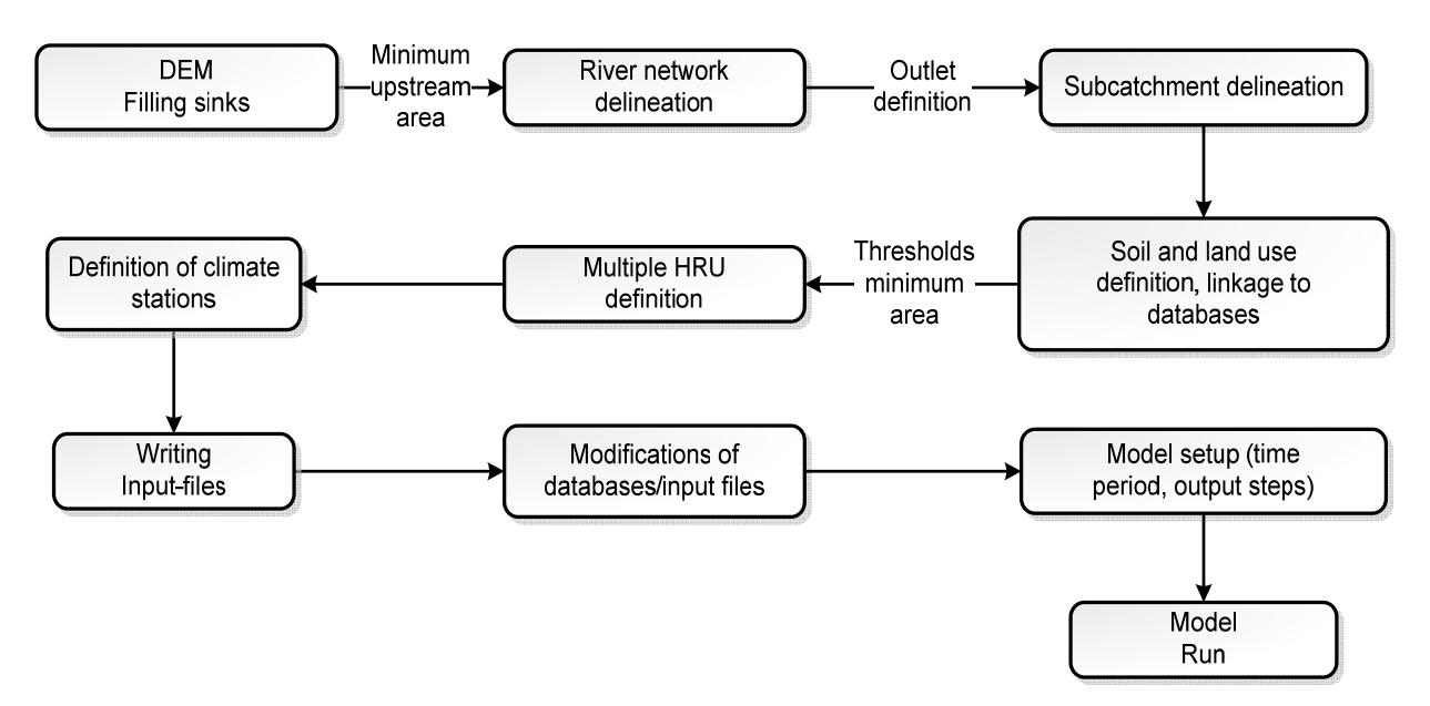
Figure 4. Steps for setting up a new SWAT project with the ArcView User Interface Source: extracted from Winchell et al, 2009
The first step to set up a SWAT model is defining elevation related parameters such as: elevations above sea level, slope aspects, river networks, distances to the adjacent rivers, and partitioning the watershed into subwatersheds. A 90 meter-resolution DEM from the Shuttle Radar Topographic Mission (SRTM) was incorpared during this step.
5.1 Baseflow separation
In order to learn about the fractions of discharge components in the measured total flow, the digital filter technique of Arnold & Allen (1999) was applied. This method was originally used in signal analysis and processing. The equation is:
\[Q_{surf}(t) = \beta \cdot Q_{surf}(t-1) + \frac{(1+\beta)}{2} \cdot \left(Q_{tot}(t) - Q_{tot}(t-1)\right)\] where:
\(Q_{surf} = \text{ filtered surface runoff (quick response)}\)
\(Q_{tot}\) = total streamflow
filter parameter (set to 0.925)
time step
Several studies have shown that the results of the digital baseflow filter compare well with manual baseflow separation techniques (Arnold & Allen 1999). The filter program delivers three baseflow curves for different climate zones. The second curve is most suitable for humid areas. Baseflow filter program is used in this study to separate baseflow from streamflow
6. Model Calibration And Evaluation
Calibration was perfored on the observed data at the watershed outlet (Nanjung gauge station) for the period of 11 years i.e from 1987 to 1997. The model performance is then evaluated on their statistical parameters, e.g. coefficient of correlation (r), coefficient of determination (R<sup>2</sup>), model efficiency (ME), and index of agreement (IA) (Spiegel, 1961).
6.1 Total water yield
Based on the comparison between the observed and simulated annual total water yield, the resulted coefficient of correlation (r) is 0.938, the coefficient of determination \((R^2)\) is 0.876, the model efficiency (ME) is 0.874 and the index of agreement (IA) is
6.2 Surface flow
Based on the comparison between the observed and simulated annual surface flow, the resulted coefficient of correlation (r) is 0.930, the coefficient of determination \((R^2)\) is 0.861, the model efficiency (ME) is 0.856 and the index of agreement (IA) is 0.962.
6.3 Base flow
Based on the comparison between the observed and simulated annual base flow, the resulted coefficient of correlation (r) is 0.893, the coefficient of determination \((R^2)\) is 0.773, the model efficiency (ME) is 0.727 and the index of agreement (IA) is 0.937.
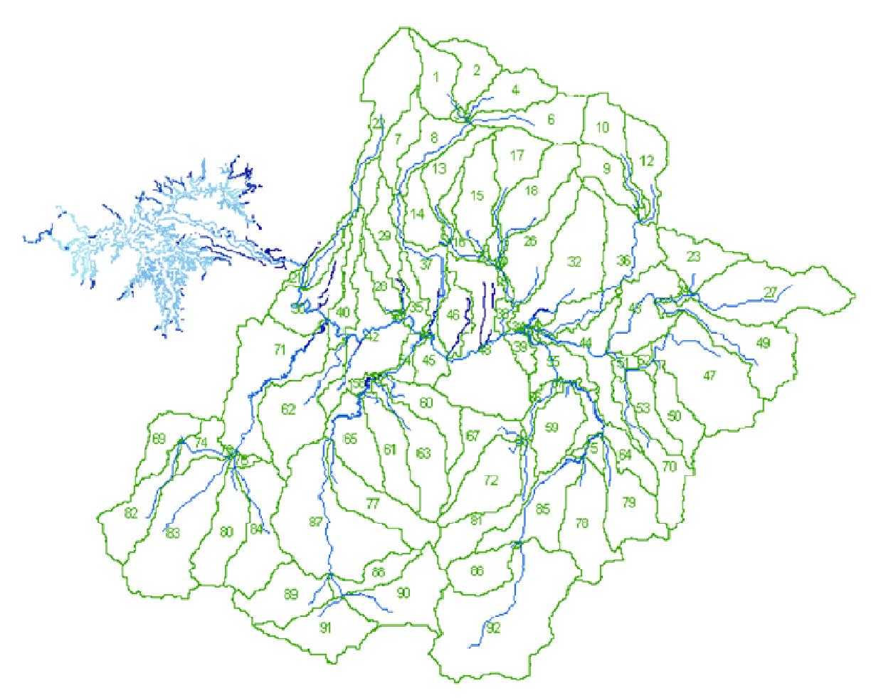
Figure 5. Watershed delineation using ArcSWAT User Interface Source: Analysis
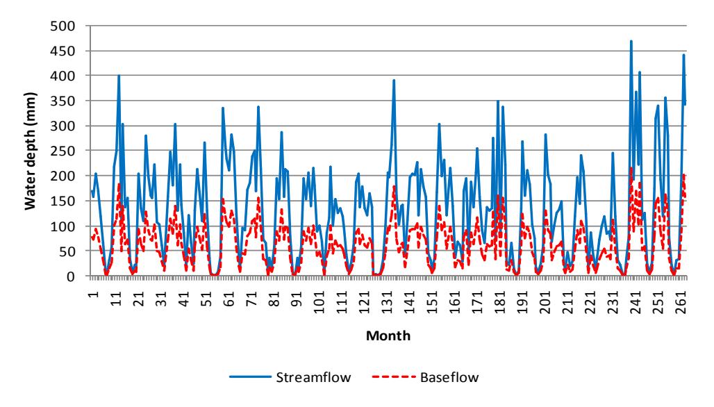
Figure 6. Baseflow separation from streamflow Source: Analysis
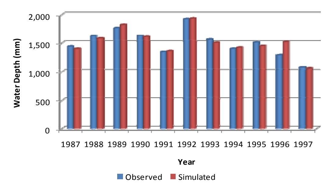
Figure 7. Calibrated annual total water yield Source: Analysis
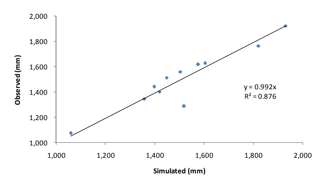
Figure 8. Relationship between simulated and observed annual total water yield Source: Analysis
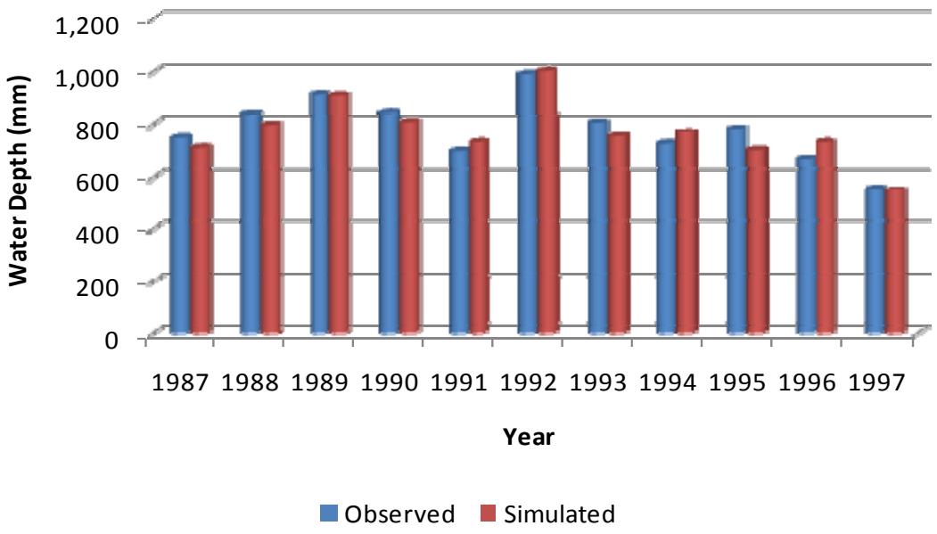
Figure 9. Calibrated annual surface flow Source: Analysis
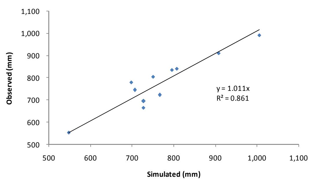
Figure 10. Relationship between simulated and observed annual surface flow Source: Analysis
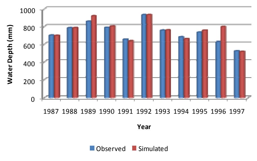
Figure 11. Calibrated annual baseflow Source: Analysis
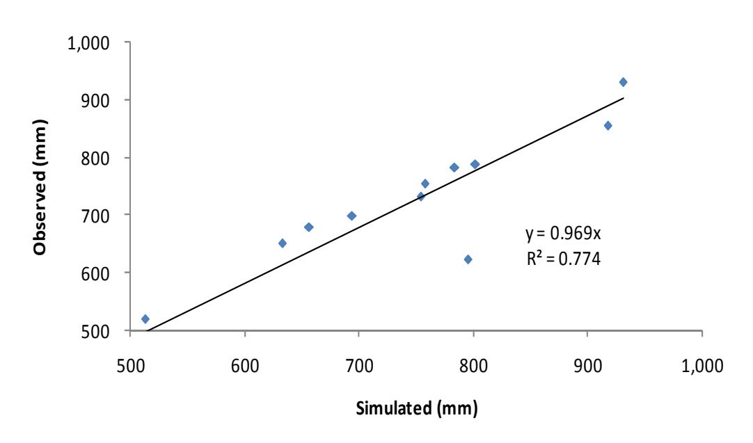
Figure 12. Relationship between simulated and observed annual baseflow Source: Analysis
6.4 Mean inflow discharge
Based on the comparison between the observed and simulated annual mean inflow discharge, the resulted coefficient of correlation (r) is 0.941 and the coefficient of determination (R2 ) is 0.883, the model efficiency (ME) is 0.878 and the index of agreement (IA) is 0.969.
6.5 Sediment Inflow
Based on the comparison between the observed and simulated annual sediment inflow, the coefficient of correlation (r) is -0.018 and the coefficient of determination (R2 ) is -0.530, the model efficiency (ME) is -0.581 and the index of agreement (IA) is 0.350. The negative values resulted because the observed annual sediment inflow is relatively constant whereas the simulated annual sediment inflow varies with the annual precipitation and mean inflow discharge.
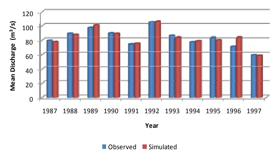
Figure 13. Calibrated annual mean inflow discharge Source: Analysis
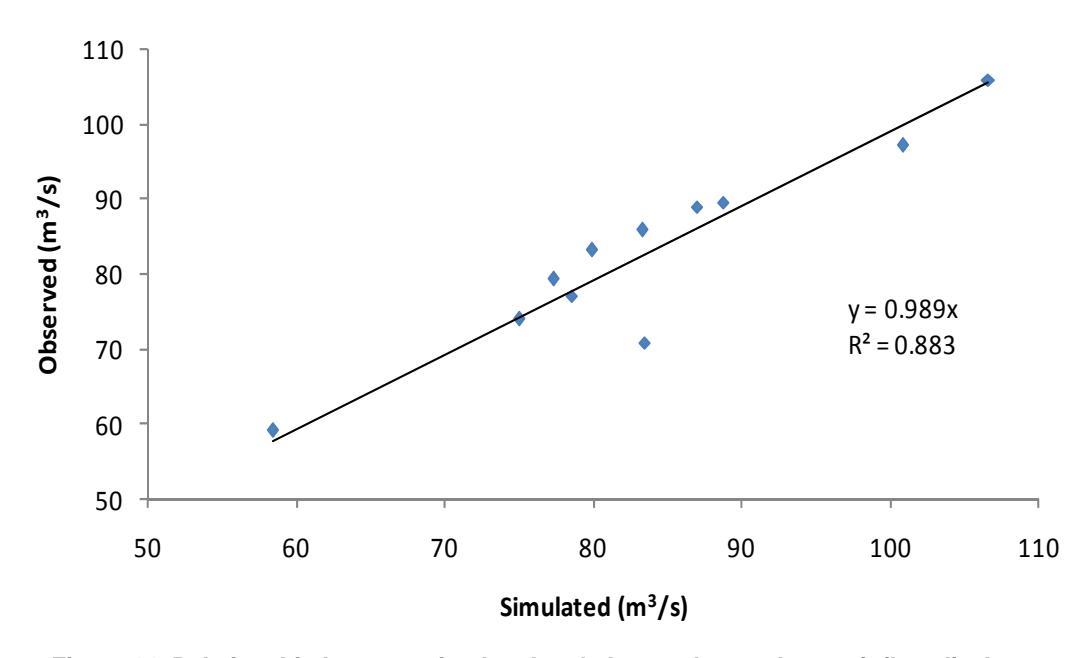
Figure 14. Relationship between simulated and observed annual mean inflow discharge Source: Analysis
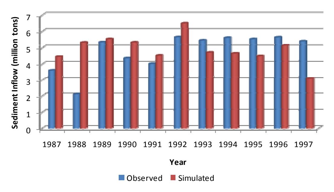
Figure 15. Calibrated annual sediment inflow Source: Analysis
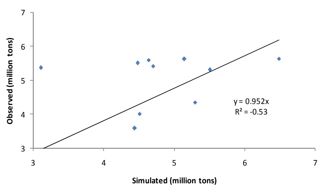
Figure 16. Relationship between simulated and observed annual mean inflow discharge Source: Analysis
The relationship between the annual mean inflow discharge and the sediment inflow is plotted in Figure 17. The deviation between the the observed and simulated interpolation lines emerges because the SWAT model accounts for the annual variation in precipitation and landuse change which is not manifested in the observed data. The observed annual sediment inflows are relatively constant regardless of the variation in the annual precipitation and mean inflow discharge.
Table 3 summarizes the mean annual values of water yield, surface flow, baseflow, inflow discharge and sediment inflow along with their statistical parameters.
Based on the calibration on the annual observed data, it was found that the model is considerably of good performance as was shown by the relatively small error and coefficient of correlation and coefficient of determination which are close to 1 except for the sediment inflow for the reason previously mentioned.
7. Model Validation And Evaluation
Validation was perfomed on the calibrated model using the consecutive 11 year data i.e. from 1998 to 2008.
Based on the validation on the annual observed values, it was found that the model is considerably of good performance as shown by the relatively small error and coefficient of correlation and coefficient of determination which are close to 1 except for the sediment inflow for the same reason as the case with the sediment inflow calibration.
8. Relationship Between The Sediment Inflow and The Critical Degree of Reservoir Lifetime
If the values of the sediment inflow (sedout) obtained from the SWAT model results and the reservoir effective lifetime obtained indirectly from Equation 6 are plotted, an exponential relationship will be issued as shown in Figure 18.
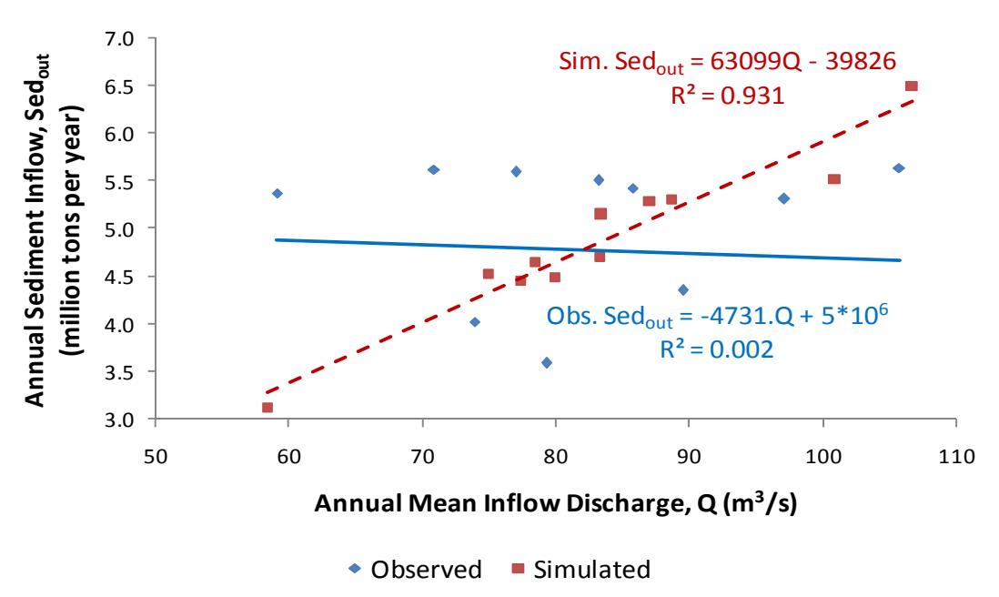
Figure 17. Relationship between annual mean inflow discharge and sediment inflow Source: Analysis
Table 3. Summary of the calibrated mean annual values
| No. | Parameter | Mean Annual Values | R2 | |||||
|---|---|---|---|---|---|---|---|---|
| Unit | Observed | Simulated | r | ME | IA | |||
| 1. | Water Yield | mm | 1,503 | 1,513 | 0.938 | 0.876 | 0.874 | 0.968 |
| 2. | Surface Flow | mm | 777 | 767 | 0.930 | 0.861 | 0.856 | 0.962 |
| 3. | Baseflow | mm | 710 | 731 | 0.893 | 0.773 | 0.727 | 0.937 |
| 4. | Inflow Discharge | m3 /s | 85.14 | 86.09 | 0.941 | 0.883 | 0.878 | 0.969 |
| 5. | Sediment Inflow | ton | 4,773,374 | 4,875,182 | -0.018 | -0.530 | -0.581 | 0.350 |
Source: Analysis
Table 4 Summary of the validated mean annual values
| No. | Parameter | Unit | Mean Annual Values | R2 | ||||
|---|---|---|---|---|---|---|---|---|
| Observed | Simulated | r | ME | IA | ||||
| 1. | Water Yield | mm | 1,628 | 1,626 | 0.987 | 0.974 | 0.974 | 0.993 |
| 2. | Surface Flow | mm | 841 | 851 | 0.967 | 0.920 | 0.914 | 0.980 |
| 3. | Baseflow | mm | 789 | 779 | 0.958 | 0.913 | 0.909 | 0.974 |
| 4. | Inflow Discharge | m3 /s | 89.61 | 89.74 | 0.988 | 0.975 | 0.976 | 0.994 |
| 5. | Sediment Inflow | ton | 5,668,783 | 5,328,818 | 0.742 | -70.500 | -70.565 | 0.272 |
Source: Analysis
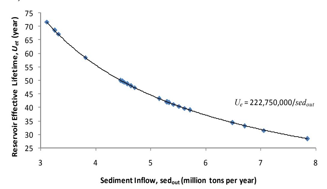
Figure 18. Relationship between the sediment inflow and the reservoir effective lifetime Source: Analysis
Thus, the reservoir effective life can be determined from the sediment inflow as:
\[U_e = \frac{222,750,000}{sed_{out}} \tag{9}\]
Similary, if the values of the reservoir efective lifetime (Ue) and the critical degree of reservoir lifetime (c) are plotted assuming the designated lifetime of 100 years, there exists an exponential relationship as shown in Figure 19.
Hence, the reservoir effective life can be determined from the sediment inflow as:
\[c = \frac{100}{U_e} \tag{10}\]
Finally, if the values of the sediment inflow (sedout) and the critical degree of reservoir lifetime (c) are plotted, a linear relationship will come up as shown in Figure 20.
From the above discussion, it can be infered that the critical degree of reservoir lifetime can be determined from the amount of sediment inflow as:
9. Conclusion
From the previous discussion it can be concluded that:
- 1. The calibration results during the period of 1987- 1997 and validation during 1998-2008 reveal that the model is considerably of good performace. This is indicated by the relatively small error and coefficient of correlation and coefficient of determination which are close to 1 except for the sediment inflow. This is due to the annual variation of precipitation and landuse change simulated in SWAT which is not manifested in the observed data. The observed annual sediment inflows are relatively constant regardless of the variation in the annual precipitation and mean inflow discharge.
- 2. From the simulation results, it is found that the mean inflow is 2,732,752,080 m3 /year
- 3. The average sediment yield is 235.86 ton/ha/year.
- 4. The mean sediment inflow is 5,102,000 tons per year which equivalent to 3,836,090 m3 which results in 46.18 year efective lifetime of the reservoir and the corresponding critical degree of 2.17.
5. The graph plotting the values of the sediment inflow and the critical degree of reservoir lifetime reveals a linear relationship.
10. Recommendation
Regarding the great number of parameters involved in the modeling process, it is recommended to conduct further research on those parameters to obtain the appropriate values in order to obtain acceptable results.
1. In Indonesia modeling using SWAT model is a new thing and scarce. It is for this reason,
- the implementation of SWAT model into the future research will be much welcomed.
- 2. To maintain the useful lifetime of the reservoir, immediate measures should be taken in order to reduce the accumulated sediment in the reservoir, e.g. by flowing the sediment out before the sedimentation taking place, building sediment control structures and conserving the ecosystem of the catchment.
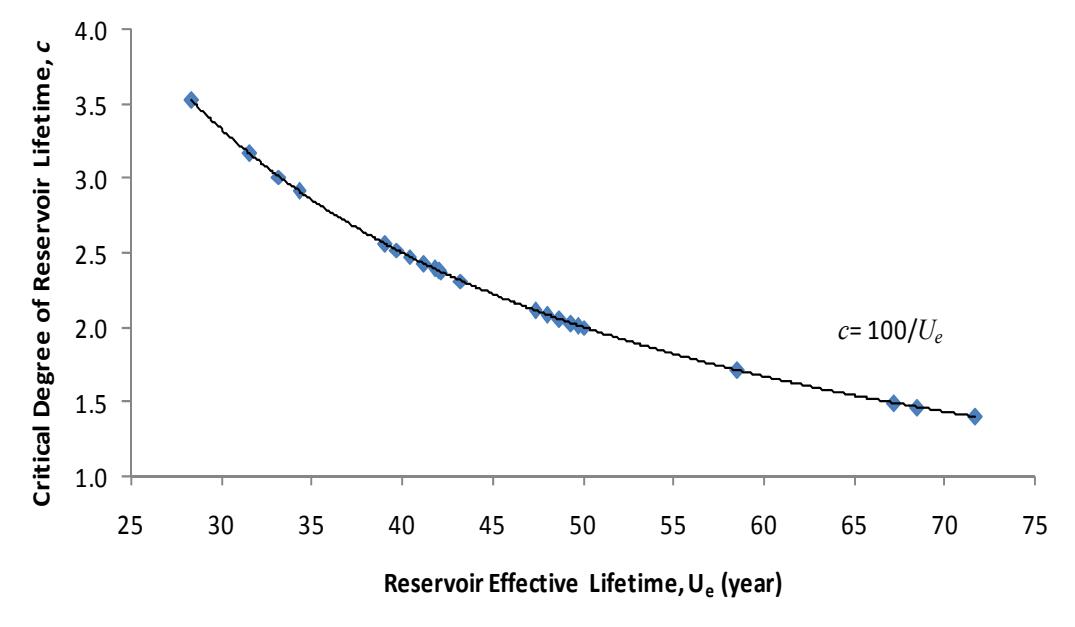
Figure 19. Relationship between the reservoir effective lifetime and the critical degree of reservoir lifetime Source: Analysis
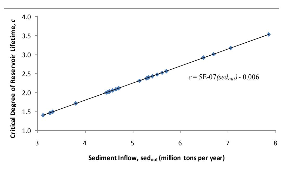
Figure 20. Relationship between the sediment inflow and the critical degree of reservoir lifetime Source: Analysis