Abstrak

Dalam studi analitik ini, algoritma paralel elemen hingga non-linier dikembangkan untuk mengatasi kelemahan dari kemampuan komputer berprosesor tunggal dalam menganalisis tanggap dinamik pada masalah interkasi antara lapisan tanah jemuh dan struktur sipil dalam skala besar. Algoritma paralel dijabarkan berdasarkam motode dekomposisi domain untuk mengubah masalah nilai batas ke masalah interfes. Metode dekomposisi domain digunakan untuk membagi keseluruhan domain yang dinalisis menjadi beberapa subdomain yang tidak saling overlap. Keungulan dari algiritma yang dikembangkan ini adalah sebagian besar proses perhitungan dilakukan dalam basis subdomain tanpa adanya komunikasi antar prosesor. Komunikasi antar prosesor hanya dilakukan ketika menyelesaikan masalah interfes. Metode iteratif Conjugate Gradient, yang digabungkan dengan komunikasi antar prosesor berbasiskan jejaring hypercube, digunakan untuk menyelesaikan masalah interfes tersebut.

Kata-kata Kunci: Metode elemen hingga non-linier 3-dimensi, paralel komputasi, metode dekomposisi domain, masalah interaksi antara lapisan tanah jenuh dan struktur sipil.

1. Introduction

The quay walls structures constructed as the waterfront structure in the port area often damaged during great earthquake. The recent example is most of quay walls constructed in the port of Kobe were damaged by the Hyogo-ken Nanbu earthquake on January 17th, 1995 (Baker and Smith, 1987). The damaged of these civil structures are indicating the complexity of the interaction problem between saturated soil layers and the civil structures. The source of complexity mostly comes from the dynamic response of the saturated soil layers where the soil grains and the pore water interacts each other.

To understand the dynamic behaviour of the waterfront structures which retain the saturated soil layers, the dynamic interaction between saturated soil layers and civil structures should be analyzed more exactly. There exist two problems for analysis the dynamic interaction problem mentioned above. The first problem is how to idealize the saturated soil layer. It is required to assume the saturated soil layer as a composite of the soil grains and the pore water. Analysis of the saturated soil layers considering the coupled system soil grains and pore water gives more realistic results compared with homogeneous equivalent solid assumption. It is also necessary to use an appropriate material constitutive model for the soil grains, which able to represent the nonlinear stress-strain relationship and the loading-unloading hysteresis loop. To solve the first problem, a simplified bounding surface plasticity model was introduced referring the previous studies by Dafalias (1986) and Crouch and Wolf (1994). In this model the change of plastic strain during cyclic loading is evaluated according to relative position of the current stress point on the loading surface inside the bounding surface. The model is applicable for both of clays and sands by unifying the parameters in the single frame of a constitutive model. The number of parameters for this model was reduced to specify the model more easily.

The second problem is how to reduce heavy loads on the computation process. Long computing time and large computer memory are needed to solve threedimensional coupling problem applying iterative method for nonlinear analysis and time history response analysis for a recorded earthquake motion. Analyses using conventional single processor very often exceed the available computer capacity. With advent the computer technology within last decades, analyzing a large-scale problem using several processor concurrently becomes possible. This type of works is called parallel computation.

There are several proposed parallel algorithms in the field of the finite element analysis as well documented in the literatures such as Tallec (1997). Papadrakakis (1997). Farhat and Raux. (1991). However, most of them were used for analyzing the homogenous or equivalent homogenous solid materials. In the previous studies, the spatial discretization for the finite element approximation was derived based on the variational method, which is not valid for the analysis of the fluid material. Therefore, in this study, the Weighted Residual Method (WRM) was applied to define the spatial discretization of the finite element and uses a shape function as the weight function as have been recommended by the Galerkin Method. WRM is more suitable for solid as well as for fluid such as a saturated soil layer.

The parallel algorithm developed herein is based the Domain Decomposition Method (DDM) (Tallec, 1997, Papadrakakis, 1997, Farhat and Raux, 1991) for separating a whole of interest domain into several non -overlapping subdomains. A traction force was used to enforce the continuity condition on the subdomain interfaces, i.e. the summation of the unknowns on the interfaces are equal to zero. As the result, a boundary value problem then can be converted into an interface

To achieve an efficient parallel algorithm, two following conditions should be considered, i.e. load works and interprocessor communication. The works in each processor should be balanced as possible and the interprocessor communication should be as less as possible. The effectiveness of the interprocessor communication is related to the scheduling and the communication algorithms (Kawamura and Tanjung, 2000). In order to reach these conditions, the proposed parallel algorithm was design to be mostly work in subdomain basis without interprocessor communication. For this purpose, the algorithm was implemented as a Single Program Multiple Data (SPMD) programming model. The interprocessor is only required when solving the interface problem.

2. Governing Equation of Motion

The governing equations of motion were derived by assuming the saturated soils compose of the soil grains and the pore water. The density of the saturated soil, \(\rho\) is expressed by the density of the soil grains \(\rho_g\)and the fluid density \(\rho_f\), as schematically shown in Figure 1.

\[\rho = (1 - v)\rho_g + f\rho_f \tag{1}\]

Assuming infinitesimal displacement, the equations of motions for saturated porous material are given as follows (Ghaboussi, 1973, Zienkiewicz, 1984).

\[\sigma_{ii,i} - \rho \ddot{\mathbf{u}}_i - \rho_f \ddot{\mathbf{w}}_i = 0 \tag{2}\]

\[p_{,i} - \rho_f \left( \ddot{u}_i + \frac{\ddot{w}_i}{f} \right) - \frac{\rho_f g}{k} \dot{w}_i = 0\] (3)

where \(\sigma_{ij}\) are the components of total stress of the saturated soil, p is the pore water pressure; u_i and w_i are the components of displacement of the soil grain and the relative displacement of the pore water to u_i. respectively. The superposed dot implies time derivative; ()_i denotes the derivative with respect to coordinates \(x_i\). For \(\sigma_{ii}\) and p tensile stresses are defined positive. k is the permeability and g is the gravitational acceleration.

where v is the porosity.

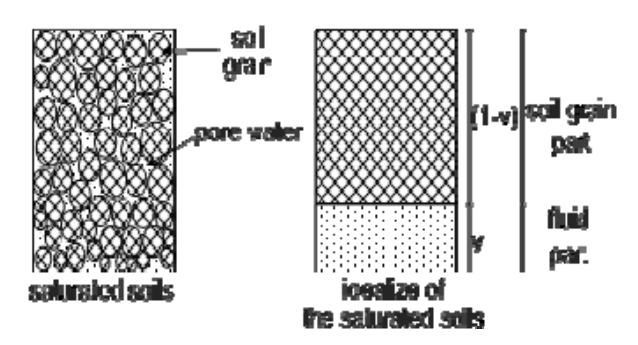
Figure 1. Idealization of saturated soils (Source: Tanjung, 2002)

3. Constitutive Model

A constitutive relation for the saturated soil layer was derived for the total stress, i.e. as a summation of the effective stress and the pore water pressure. For the pore water, the constitutive relation was obtained by applying the mass conservation law to the flow of the pore water in saturated soil layer. Their increment form is given as follow (Dafalias, 1986).

\[\dot{\sigma}_{ij} = D_{ijkl} \ \dot{\epsilon}_{kl} + \alpha^2 \ \delta_{ij} K_{gf} \delta_{kl} \ \dot{\epsilon}_{kl} + \alpha \ K_{gf} \delta_{ij} \ \dot{\zeta} \eqno(4)\]

\[\dot{p} = K_{gf} \left( \alpha \, \dot{\epsilon}_{ii} + \dot{\zeta} \right) \tag{5}\]

\[\frac{1}{K_{gf}} = \frac{1}{K_g} + \frac{1}{K_f}\] (6)

\[\alpha = 1 - \frac{\delta_{ij} D_{ijkl} \delta_{kl}}{3K_g}\] (7)

\(\dot{\sigma}_{ii}\) and \(\dot{p}\) are the total stress and pore water pressure

increment, respectively. \(K_g\), \(K_f\) and \(K_{gf}\) are the bulk modulus for the soil grain, pore water and their coupling, respectively, \(\alpha\) is a measure of compressibility of the soil grains representing the contact areas of the soil grains to pore water. Dijkl represents the stressstrain relation of soil grain. di is the component of the Kronecker's delta.

\(\dot{\epsilon}_{ii}\) and \(\dot{\zeta}\) are the strain of soil grain and volumetric

strain of the pore water increments, respectively. By using the small deformation theory, their values are defined as follow.

\[\dot{\varepsilon}_{ij} = \frac{1}{2} \left( \mathbf{u}_{i,j} + \mathbf{u}_{j,i} \right) \tag{8}\]

\[\dot{\zeta} = \mathbf{w}_{i,i} \tag{9}\]

Elastoplastic stress-strain relation \(D_{iikl}^{ep}\) for the general

type of yield function may be expressed as following equation (Dafalias, 1986).

\[D_{ijkl}^{ep} = D_{ijkl}^{e} - u(L) \frac{D_{ijmn}^{e} P_{mn} Q_{pq} D_{pqkl}^{e}}{H + Q_{ab} D_{abcd}^{e} P_{cd}}\](10)

in which

\[L = \frac{Q_{ij} D_{ijkl}^e \dot{\varepsilon}_{kl}}{H + Q_{ab} D_{abcd}^e P_{cd}}\](11)

\[P_{ij} = \frac{\partial g_p}{\partial \sigma'_{ij}}\] (12)

\[Q_{ij} = \frac{\partial f}{\partial \sigma'_{ij}}\] (13)

D^e_iikl represents the elastic stress-strain relation, H is the plastic hardening modulus, gp and f are the plastic potential and the yield functions. u(L) is the heavy-step function, u(L)=1 for \(L \ge 0\) and u(L)=0 for L<0. In the bounding surface plasticity model, these relations are applied not only for the bounding surface but also for the loading surface inside the bounding surface. To specify the relations in Equation 10 in detail, the definition of the elastic stress-strain relation \(D^e_{ijkl}\), the failure surface F_f, the bounding surface F_b, the loading surface f_L and the plastic strain potential g_p should be determined. The form of the functions mentioned above is explained in the followings.

3.1 Elastic stress-strain relation

The elastic stress-strain relation \(D_{ijkl}^e\) is expressed as

\[D_{ijkl}^{e} = 2G \, \delta_{ik} \delta_{jl} + \left( K_g - \frac{2}{3} G \right) \delta_{ij} \delta_{kl}\] (14)

The notation \(K_g\) and G denote bulk and shear modulus of the soil grains, respectively. They are defined based on the critical state of soil mechanics concept as written in the following expressions for a given constant Poisson's ratio v.

\[\frac{K_g}{p_a} = \frac{1 + e_{in}}{\kappa} \left(\frac{I}{3p_a}\right)^{0.5} \tag{15}\]

\[G = \frac{3(1-2v)}{2(1+v)} K_g\] (16)

Notation \(e_{in}\) indicates the initial void ratio, \(\kappa\) is the slope of the swelling process in the consolidation curve, pa is the atmosphere pressure, I is the first invariant of stress

3.2 Failure surface

An expression for failure surface F_f is defined as

\[F_{f} = -\zeta_{cr}I + J = 0 \tag{17}\]

J is the second invariant of deviatoric stress; V_cr is the slope of the critical state line in the meridional section shown in Figure 3. In the effective stress space, the critical state is represented by an elliptic cone function \(\rho_c\) as proposed by Crouch and Wolf (1994) as follow.

\[\varsigma_{\rm cr} = \rho_{\rm c} \frac{2 \sin \phi_{\rm cr}}{\sqrt{3} \left( 3 - \sin \phi_{\rm cr} \right)} \tag{18}\]

The shape of the cone is shown in Figure 2. The shape of the cone is controlled by the Lode angle \(\theta\) and a material parameter defining the compression critical friction angle \(\phi_{er}\).

3.3 Bounding surface

A single elliptic surface shown in Figure 3 was used as the bounding surface in this study. The parameter R controls the aspect ratio of the ellipse. The form of the bounding surface \(F_b\) is given in following equation (Tanjung, 2002).

\[F_{b} = \overline{J}^{2} - \frac{(\varsigma_{cr} I_{0})^{2}}{R^{2}} \left( 1 - \frac{1}{(R-1)^{2}} \left( \frac{R\overline{I}}{I_{0}} - 1 \right)^{2} \right) = 0\] (19)

Figure 2. Elliptic cone shape of failure surface (Source: 2.Crouch, at.al., 1994)

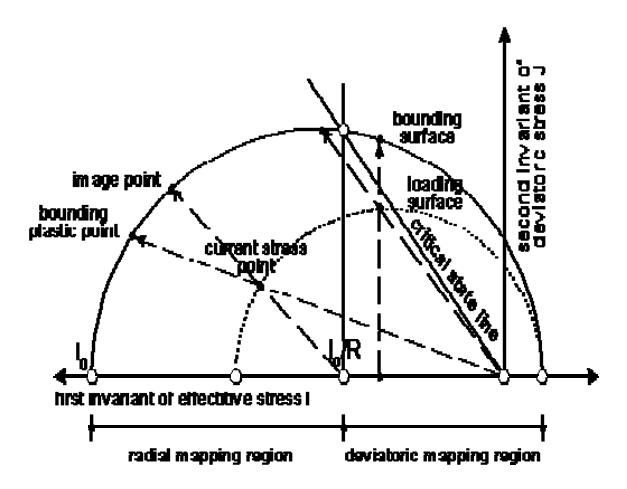
Figure 3. Single elliptic of bounding surface model (Source: Tanjung, 2002)

The size of bounding is defined by a maximum isotropic compression stress \(I_0\). The bounding surface moves during plastic flow and always envelopes the current effective stress state. The evolution of the bounding surface depends on the volumetric plastic strain increment \(\varepsilon^{\cdot p}_{\nu}\) as expressed in Equation (20). The bounding surface may expand or shrink depends upon whether the plastic volumetric \(\varepsilon^{\cdot p}_{\nu}\) increases or decreases.

\[\frac{\dot{I}_0}{p_a} = \frac{1 + e_{in}}{\lambda_c - \kappa} \left( \frac{I_0}{3p_a} \right) \dot{\varepsilon}_v^p \tag{20}\]

\(\lambda_c\) is a slope of isotropic consolidation line.

3.4 Loading surface

A loading surface is required to define the loading direction and to evaluate the plastic condition on the current effective stress point. The shape of the loading surface was taken similar with the bounding surface form. The plastic condition of the loading surface, which is located inside the bounding surface, is related to the plastic condition on the bounding surface.

\[(\overline{1},\overline{J})\] on the bounding surface. In order to capture

As shown in Figure 3, this relation is taken by mapping the current stress point (I,J) to the image point the wide range of the soil responses, the following combination of radial and deviatoric mapping rules have been applied (Tanjung, 2002).

\[\overline{I} = \left(\frac{I_0}{R}\right) + \beta \left(I - \frac{I_0}{R}\right); \ \overline{J} = \beta J \ ; \text{ for } I < I_0 / R\] (radial mapping) (21)

\[\overline{I} = I\]; \(\overline{J} = \beta J\) for \(I \ge I_0 / R\) (deviatoric mapping) (22)

A constant \(\beta\) called a similarity ratio. The equations which define the loading surfaces in the radial and deviatoric mapping regions can be obtained by substituting Equations 21 and 22 into the bounding surface equation, Equation 19, respectively.

\[f_{L} = \beta^{2} J^{2} - \frac{\left(\varsigma_{cr} I_{0}\right)^{2}}{R^{2}} \left(1 - \frac{\beta^{2}}{\left(R - 1\right)^{2}} \left(\frac{RI}{I_{0}} - 1\right)^{2}\right) = 0 \quad (23)\]

\[f_{L} = \beta^{2} J^{2} - \frac{\left(\varsigma_{cr} I_{0}\right)^{2}}{R^{2}} \left(1 - \frac{1}{\left(R - 1\right)^{2}} \left(\frac{RI}{I_{0}} - 1\right)^{2}\right) = 0 \quad (24)\]

3.5 Potential surface

The potential surface g_p is also assumed as the similar form with the bounding surface.

\[g_p = J^2 - \frac{\left(\varsigma_{cr} I_{0g}\right)^2}{R^2} \left(1 - \frac{1}{\left(R - 1\right)^2} \left(\frac{RI}{I_{0g}} - 1\right)^2\right) = 0 (25)\] in which subscript g denotes the parameters related to the potential surface \(g_p\). All parameters except \(I_{0g}\) are same with those of the bounding surface. A parameter \(I_{0g}\) is scaled such that the current stress point lies on the potential surface. Although the bounding, the loading and the potential surfaces are the similar elliptic form, these surfaces are not geometrically identical and the responses of the soil are always obtained in the nonassociated flow rule.

3.6 Plastic hardening modulus

The consistency condition for the yield surface is required to maintain the effective stress point always lies within or on the yield surface. For the bounding surface plasticity model, the consistency condition is applied to the bounding surface function F_b. The plastic hardening modulus H on the loading surface is defined referring the value of the plastic hardening modulus

H on the bounding surface.

\[H = \overline{H} + H_f \tag{26}\] in which \(\overline{H}\) is evaluated by the following equation.

\[\overline{H} = -\frac{1 + e_{in}}{\lambda - \kappa} I_0 \frac{\partial F}{\partial I_0} P_{ii}\] (27)

A term \(\partial F/\partial I_0\) is considered for the bounding plastic point on the bounding surface. Its point is determined by projecting the current stress point from the origin of the stress space onto the bounding surface using the following mapping rule.

\[\overline{I} = \beta I; \ \overline{J} = \beta J\] (28)

As was previously mentioned, the feature of the bounding surface plasticity model is that the plastic strain is allowed to occur not only on the bounding surface, but also inside the bounding surface. This plastic strain inside the bounding surface can be considered as the relative plastic strain to the plastic strain on the bounding surface. To take into account the plastic strain inside the bounding surface, Crouch and Wolf (1994) proposed an additional plastic hardening modulus H_f as

\[H_{f} = \frac{1 + e_{in}}{\lambda - \kappa} \frac{h}{\langle \beta / (\beta - 1) - s_{e} \rangle} \left( \frac{I_{0}}{3p_{a}} \right)^{1.5}\] (29)

A constant h is a material parameter represents the hardening behaviour of the soil grains and parameter S_e defines the elastic nucleus where an only elastic strain is developed.

4. Nonlinear Dynamic Parallel

4.1 Applied DDM in FEM Formulation

To clarify usage of a Domain Decomposition Method (DDM) in the nonlinear FEM formulation, consider a case of a domain \(\Omega\) separated into two totally nonoverlapping subdomains \(\Omega^{(1)}\) and \(\Omega^{(2)}\) shown in Figure 4. Extrapolation to number of Ns subdomains can be done in a straightforward. The \(\Gamma^{(12)}\) is the interface between subdomain \(\Omega^{(1)}\) and subdomain \(\Omega^{(2)}\). Under constraint of the displacements field on the interface the additional boundary condition as written in Equation 30 is required with the continuity condition given in Equation 31 (Kawamura and Tanjung, 2000, Kawamura and Tanjung, 2001).

\[\begin{cases} \lambda_{ij}^{u} n_{j} \\ \lambda_{ij}^{w} n_{j} \end{cases}^{(1)} + \begin{cases} \lambda_{ij}^{u} n_{j} \\ \lambda_{ij}^{w} n_{j} \end{cases}^{(2)} = 0 \quad \text{on } \Gamma^{(12)}\] (30)

\(\lambda_{ii}\) denotes a traction tensor and \(n_i\) is an outer normal

A solution of the above problem is obtained by applying the Weighted Residual Method (WRM) (Zienkiewicz and Taylor, 1991, Hughes, 1996) to the governing equations of motion (2) and (3), the continuity condition on the interface (31) and the boundary condition (30).

Figure 4. Decompose into two subdomains (Source: Tanjung, 2002)

\[\text{[rumus tidak dapat ditampilkan dengan baik — lihat PDF asli]}\] \[(32)\]

\[\int_{\Gamma^{(12)}} \left\{ \delta \lambda_{ij}^{u} \ n_{j} \ \delta \lambda_{ij}^{w} \ n_{j} \right\}^{(12)} \left\{ \begin{cases} u_{i} \ n_{j} \\ w_{i} \ n_{j} \end{cases}^{(1)} - \begin{cases} u_{i} \ n_{j} \\ w_{i} \ n_{j} \end{cases}^{(2)} \right\} d\Gamma^{(12)} = 0\] (33)

Superscript (s) denotes the subdomain number, \(\delta u_i\) and δw_i are the arbitrary functions which represent the weight for approximating the values of the displacements u_i and w_i. It is possible to reduce an order of differentiation in the first term of left hand side of Equation 32 via integration by parts of Green's theorem. The spatial discretization for the finite element is then obtained by introducing the weight function for Equation 32 and 33. The Galerkin method (Zienkiewicz and Taylor, 1991, Hughes, 1996) was applied in this study; i.e. uses an original shape function as a weight function. The final equation of motion for the finite element analysis is obtained as written in Equation 34.

\[\sum_{s=1}^{2} \left[ \mathbf{M}^{(s)} \ddot{\mathbf{d}}^{(s)} + \mathbf{D}^{(s)} \dot{\mathbf{d}}^{(s)} + \mathbf{K}^{(s)} \dot{\mathbf{d}}^{(s)} \right] = \sum_{s=1}^{2} \left[ \mathbf{F}^{(s)} - \mathbf{B}^{(s)^{T}} \boldsymbol{\lambda} \right]\] (34)

with respect to continuity condition,

\[\sum_{s=1}^{2} \mathbf{B}^{(s)} \mathbf{d}^{(s)} = \mathbf{0}\] (35)

in which

\[\boldsymbol{d}^{(s)} = \begin{cases} \boldsymbol{d}_u^{(s)} \\ \boldsymbol{d}_w^{(s)} \end{cases}; \boldsymbol{M}^{(s)} = \begin{bmatrix} \boldsymbol{M}_u^{(s)} & \boldsymbol{M}_c^{(s)} \\ \boldsymbol{M}_c^{(s)^T} & \boldsymbol{M}_w^{(s)} \end{bmatrix}; \boldsymbol{D}^{(s)} =\]

\[\begin{bmatrix} \mathbf{D}_{\mathrm{u}}^{(\mathrm{s})} & 0 \\ 0 & \mathbf{D}_{\mathrm{w}}^{(\mathrm{s})} \end{bmatrix}; \mathbf{K}^{(\mathrm{s})} = \begin{bmatrix} \mathbf{K}_{\mathrm{Tu}}^{(\mathrm{s})} & \mathbf{K}_{\mathrm{c}}^{(\mathrm{s})} \\ \mathbf{K}_{\mathrm{c}}^{(\mathrm{s})^{\mathrm{T}}} & \mathbf{K}_{\mathrm{w}}^{(\mathrm{s})} \end{bmatrix}\]

\(\mathbf{M}^{(s)}\), \(\mathbf{D}^{(s)}\) and \(\mathbf{K}^{(s)}\) are the mass, damping and stiffness matrices for each subdomain. \(K^{(s)}_{Tu}\) is the tangent stiffness matrix for the soil grains part, which depends on the effective stress history. The detailed formulation of these matrices for an 8-node brick element was written in reference (Kawamura and Tanjung, 2000). The subscript u and w denotes the soil grains and the pore water, respectively, the subscript c designates the coupling condition. The vectors \(d_u^{(s)}\) and \(d_w^{(s)}\) are the relative displacement of the soil grains and the pore water to the ground motion, respectively. The vector \(\lambda\) is composed of \(\lambda_{ij}\) which is traction forces on the interface nodes. The matrix B(s) is signed Boolean matrix, which localizes a subdomain quantity to the subdomain interface. If the interior degrees of freedom are numbered first and the interface ones are numbered last, the Boolean matrix B^(s) takes a form,

\[\mathbf{B}^{(s)} = \begin{bmatrix} \mathbf{0} & \mathbf{I} \end{bmatrix} \tag{36}\]

In above equation, 0 and I denote a null and identity matrices.

4.2 Numerical solution of the equation of motion

Perhaps the most widely used the direct time integrating method for solving the equation of motion such as written in Equation 34 is the Newmark's family (Newmark, 1959). In this study, the Hilber-α (Hughes, 1996) method has been used. In this study, the following approximation was used to integrate equation of motion for constant increment time step Dt following the Hilber-α method.

\[\mathbf{d}_{n}^{(s)} = \mathbf{d}_{n-1}^{(s)} + \Delta \mathbf{d}_{n}^{(s)} \tag{37}\]

\[\dot{\boldsymbol{d}}_{n}^{(s)} = \frac{\overline{\gamma}}{\overline{\beta} \Delta t} \Delta \boldsymbol{d}_{n}^{(s)} + \left(1 - \frac{\overline{\gamma}}{\overline{\beta}}\right) \dot{\boldsymbol{d}}_{n-1}^{(s)} + \left(1 - \frac{\overline{\gamma}}{2\overline{\beta}}\right) \Delta t \ \ddot{\boldsymbol{d}}_{n-1}^{(s)}\]

\[\ddot{\mathbf{d}}_{n}^{(s)} = \frac{1}{\overline{\beta} \Delta t^{2}} \Delta \mathbf{d}_{n}^{(s)} - \frac{1}{\overline{\beta} \Delta t} \dot{\mathbf{d}}_{n-1}^{(s)} + \left(1 - \frac{1}{2\overline{\beta}}\right) \ddot{\mathbf{d}}_{n-1}^{(s)}\] (39)

The parameters \(\bar{\alpha}\), \(\bar{\gamma}\) and \(\bar{\beta}\) are specified as follow.

\[\frac{1}{3} \le \overline{\alpha} \le 0; \ \overline{\gamma} = \frac{1 - 2\overline{\alpha}}{2}; \ \overline{\beta} = \frac{\left(1 - \overline{\alpha}\right)^2}{4}\] (40)

At first, subscripts n and k in the equations of motion (34) and (35) are introduced for signing a time step and nonlinear iteration number.

Substituting Equations 37 to 39 into Equations 34

\[\sum_{s=1}^{Ns} \left[ \hat{\boldsymbol{K}}_{T_n}^{(s)}^{(s)} \Delta \boldsymbol{d}_n^{(s)} \right] = \sum_{s=1}^{Ns} \left[ {}^{(k)} \Delta \boldsymbol{R}_n^{(s)} - \boldsymbol{B}^{(s)^T}^{(s)} \Delta \boldsymbol{\lambda}_n \right]\] and 35 lead to following expression. The Equations 41 to 43 have been extended to Ns subdomains instead of 2 subdomains derived in foregoing

\[\sum_{s=l}^{Ns} \left[ \boldsymbol{B}^{(s)} \hat{\boldsymbol{K}}_{T_n}^{(s)^{-l}} \boldsymbol{B}^{(s)^T} \right]^{(k)} \Delta \boldsymbol{\lambda}_n = \sum_{s=l}^{Ns} \left[ \boldsymbol{B}^{(s)} \hat{\boldsymbol{K}}_{T_n}^{(s)^{-l}}^{(k)} \Delta \boldsymbol{R}_n^{(s)} \right]\]

with respect to continuity condition

\[\sum_{s=1}^{Ns} \mathbf{B}^{(s)} {}^{(k)} \Delta \mathbf{d}_{n}^{(s)} = \mathbf{0} \text{ mulations.}\] (43)

where A boundary value problem written in Equation 47 may be converted into following inter-

\[\hat{\mathbf{K}}_{T_{n}}^{(s)} = \frac{1}{\overline{\beta} \Delta t^{2}} \mathbf{M}^{(s)} + \frac{\overline{\gamma}}{\overline{\beta} \Delta t} \mathbf{D}_{n-I}^{(s)} + \mathbf{K}_{T_{n-1}}^{(s)}\](44)

\[{}^{(k)}\Delta\mathbf{R}_{n}^{(s)} = \hat{\mathbf{F}}_{n}^{(s)} - \sum_{i=1}^{k-l} \left( \hat{\mathbf{K}}_{T_{n}}^{(s)} {}^{(j)} \Delta\mathbf{d}_{n}^{(s)} \right)^{\text{lem.}}\](45)

\[\Delta \hat{\mathbf{F}}_{n}^{(s)} = \left(\mathbf{F}_{n}^{(s)} - \mathbf{F}_{n-1}^{(s)}\right) + \left(\frac{1}{\overline{\beta}} \Delta t \mathbf{M}^{(s)} + \frac{\overline{\gamma}}{\overline{\beta}} \mathbf{D}_{n-I}^{(s)}\right) \dot{\mathbf{d}}_{n-1}^{(s)}\]\[+ \left(\frac{1}{2\overline{\beta}} \mathbf{M}^{(s)} + \left(\frac{\overline{\gamma}}{2\overline{\beta}} - 1\right) \Delta t \mathbf{D}_{n-I}^{(s)}\right) \ddot{\mathbf{d}}_{n-1}^{(s)}\] (46)

Obviously, there are three unknowns which have to be solved in the equation of motion (41), i.e. \(K^{(s)}_{Tn}\), \(k^{(k)}\Delta\lambda_n\)

\[^{(k)}\Delta \mathbf{d}_{n}^{(s)} = \hat{\mathbf{K}}_{T_{n}}^{(s)^{-1}} \begin{pmatrix} {}^{(k)}\Delta \mathbf{R}_{n}^{(s)} - \mathbf{B}^{(s)^{T}} & {}^{(k)}\Delta \boldsymbol{\lambda}_{n} \end{pmatrix}\](47)

and \({}^{(k)}\Delta d^{(s)}_{n}\). According to the Modified Newton-Raphson Method (Press, 1995) applied for solving the nonlinear condition in this study; a current tangent stiff-

\[\frac{(k) \Delta \boldsymbol{R}_{n}^{(s)^{T}} \sum_{j=1}^{k} (j) \Delta \boldsymbol{d}_{n}^{(s)}}{\Delta \hat{\boldsymbol{F}}_{n}^{(s)^{T}} \sum_{j=1}^{k} (j) \Delta \boldsymbol{d}_{n}^{(s)}} \leq \epsilon_{c}^{\text{ness matrix } K^{(s)}_{Tn} \text{ may be approximated by a known previous value } K^{(s)}_{tn-1} \text{ An iterative solver of the Conjugate Gradient (CG) algorithm}}\]

(Gill and Murray, 1974) explained in following subsection is employed for defining an increment of traction forces^(k)\(\Delta \lambda_n\). After ^(k)\(\Delta \lambda_n\) has been obtained, the increment of displacement vector for each subdomain at current iteration (k) \(\Delta d^{(s)}_{n}\) can be

\[\Delta \mathbf{d}_{n}^{(s)} = \sum_{k=1}^{nk} {k \choose k} \Delta \mathbf{d}_{n}^{(s)} \quad \text{evaluated by the following}\] equation. (49)

The iterative process in the Newton-Raphson algorithm is terminated when the following convergence criterion in each subdomain is satisfied.

Where \(\varepsilon_c\) is a convergence criterion constant. If nk is a number of converged Newton-Raphson iteration, the increment of displacement vector for current time

\[{}_{n}\Delta \sigma_{ ij}={}_{n}D^{ e p}_{ijkl}\ {}_{n}\Delta \epsilon_{kl}+{}_{n}\alpha^{2}\delta_{ij}\,{}_{n}K_{gf}\delta_{kl}\ {}_{n}\Delta \epsilon_{kl}+{}_{n}\alpha \delta_{ij}\ {}_{n}\Delta \zeta\]

step is defined as follow, (50)

\[{}_{n}\Delta p = {}_{n}K_{gf} \left( {}_{n}\alpha {}_{n}\Delta \varepsilon_{ii} + {}_{n}\Delta \zeta \right)\] (51)

\[{}_{n}\Delta\sigma'_{ij} = {}_{n}\Delta\sigma_{ij} - \delta_{ij} {}_{n}\alpha {}_{n}\Delta p\] (52)

Finally, the dynamic in which, response for each subdomain at current time

\[_{n}\alpha=1-\frac{\delta_{ij\;n}D_{ijkl}^{ep}\delta_{kl}}{3K_{g}}\] step can be computed using
Equation 37, 38 and
39 for displacement, velocity and accelera-

\[\frac{1}{{}_{n}K_{gf}} = \frac{f}{K_{f}} + \frac{{}_{n}\alpha - f}{K_{g}}\] tion, respectively.
For a given strain increment of the soil grains \({}_{n}\Delta\epsilon_{ii}\)

and the volume change of the pore water \(_{n}\Delta\zeta\), which are evaluated based on the Equation 8 and 9, respectively, the increment of the stresses state can be calculated according to the Equation 4 and 5. In numerical analysis, the evaluation of these stresses is conducted as in Equation 50 to 54. In these equations a notation \(\Delta\) for denoting the increment is introduced instead of superposed dot used in Equation 4 and 5.

\[_{n}D_{ijkl}^{ep} = \frac{1}{2} \left( {_{n-l}D_{ijkl}^{ep} + _{n}^{p}D_{ijkl}^{ep}} \right)\] (55)

\[{}_{n}^{p}\sigma'_{ij} = {}_{n-1}\sigma'_{ij} + {}_{n}^{p}\Delta\sigma'_{ij}\] (56)

The stresses state increment at current are depending on the unknown quantity of the elastoplastic stressstrain relation for soil grains _nD^ep_iikl. In order to find the answer of the stresses state increment equations 50 to 52, a local iteration has been introduced. For this purpose, the elastoplastic stress-strain relation for the soil grains _nD^ep_ijkl is approximated as follows (Tanjung, 2002).

A _n-1 D^ep_ijkl is the elastoplastic stress-strain relation for the soil grains defined based on the effective stress \(_{n-1}\sigma'_{ij}\) on the previous time step (n-1). Superscript p in the second term of Equation 55 denotes it elastoplastic stress-strain relation evaluated according to a predicted effective stress below.

The predicted effective stress increment \({}^{p}_{n}\Delta\sigma'_{ii}\) is approximated based on the value of the effective stress increment on the previous local iteration. Both of elastoplastic stress-strain relations for the soil grains written in the right hand side of Equation 55 are evaluated using the simplified bounding surface plasticity model previously mentioned. The local iteration process is terminated when a ratio of the norm of the residual of the predicted effective stress increment \({}^{p}_{n}\Delta\sigma'_{ii}\) to the effective stress increment n _nΔσ'_ij goes vanishing.

4.3 Parallel computation algorithm

Most of the computations for the Parallel FEM formulations developed in the previous subsection can be performed in the subdomain basis. These computations are identical with the works in the conventional finite

element analysis, such as forming and assembling mass matrix \(\mathbf{M}^{(s)}\), damping matrix \(\mathbf{D}^{(s)}\), tangential stiffness matrix \(K^{(s)}_{Tu}\), the dynamic loading vector \(\mathbf{F}^{(s)}\)and evaluating equations 50 to 62. When these works are assigned to the individual processors in the multiprocessors machine, each processor will performs an identical works as above. The different work in each processor is only related to the properties of the considered subdomain. Each processor will analyze a subdomain according to it own input data. When the computations have terminated, each processor will also record it own results. Since each processor conducts the identical works, we only need to develop a single algorithm flow as the usual finite element analysis. The algorithm may be executed in the assigned processor. A special treatment is only required to manage the algorithm for perthat the components of matrix-matrix \(\left[\mathbf{B}^{(s)}\hat{\mathbf{K}}_{T_n}^{(s)^{-1}}\mathbf{B}^{(s)^{T}}\right]\)forming the computations with respect to the different input data - related to the different properties of the subdomains – on the different processors. When the processors need to exchange the since the components of matrix \[\mathbf{B}^{(s)}\hat{\mathbf{K}}_{T_n}^{(s)^{-1}}\mathbf{B}^{(s)^T}\] are data with other processors, the processors can explicitly send and/or receive to and/or from other processors. This type of programming model is known as Single Program Multiple Data (SPMD) programming model (Kawamura and Tanjung, 2000, Tanjung, 2002, Baker and Smith, and the initial residual vector \[\mathbf{r}_0 = \mathbf{B}^{(s)} \hat{\mathbf{K}}_{T_n}^{(s)^{-1}} \hat{\mathbf{k}} \Delta \mathbf{R}_n^{(s)}\] 1987, Kumar, 1994). Another different point to a sequential programming model is only related to the interprocessor communication. This interprocessor communication only takes

place

\[\begin{aligned} & \mathbf{z}_{i-l} = \overline{\mathbf{A}}_{\mathbf{I}}^{\mathbf{-1}} \ \mathbf{r}_{i-l} & \text{when} \\ & \boldsymbol{\zeta}_{i} = \mathbf{z}_{i-1}^{T} \ \mathbf{r}_{i-l} \big/ \mathbf{z}_{i-2}^{T} \ \mathbf{r}_{i-2} & (\boldsymbol{\zeta}_{1} = \boldsymbol{0}) & \text{an interface} \\ & \mathbf{s}_{i} = \mathbf{z}_{i-l} + \boldsymbol{\zeta}_{i} \ \mathbf{s}_{i-l} & (\mathbf{s}_{0} = \mathbf{z}_{0}) & \text{prob-} \end{aligned}\] \[\text{[rumus tidak dapat ditampilkan dengan baik — lihat PDF asli]}\]

A term of \(\overline{\mathbf{A}}_{1}^{-1}\) in the CG algorithms (57) above is tioned above, the traction vector (k)Dl_n is defined by converting the boundary value problem into an interface problem as written in Equation 42. It problem is

\[\bar{\mathbf{A}}_{I}^{-1} = \sum_{s=1}^{Ns} \begin{bmatrix} \mathbf{0} & \mathbf{0} \\ \mathbf{0} & \bar{\mathbf{K}}_{bb}^{(s)} \end{bmatrix}\] identical to a minimizing problem respect to continuity condition given in Equation 43 In this study, an iterative solver of the Conjugate Gradient (CG) algorithm was used to solve its interface problem. One of the features of the CG method is in this study - are maintained without modification during iteration. This feature is very convenient to solve the minimizing problem in the parallel machine constructed in the several independent individual processors. Specifically, the algorithm of CG method goes as follow. A superscript k traction vector \(^{(k)}\Delta\lambda_n\)is temporary omitted for simplification. The initial value of the tractor vector \(\lambda_0\) is given as a null vector; \(l_0 = 0\)

The following calculations are iterated until convergence criterion is confirmed (Kawamura and Tanjung, 2000, Tanjung, 2002).

known as a preconditioner. The preconditioner is used to enhance the convergence rate. The form of the preconditioner is written in Equation 58 following the form proposed by Farhat (1991).

The solution of the interface problem requires interprocessor communication such that the data can be exchanged from one processor to others. In fact this exchanged data significantly affects the parallel computing performance, since the communication will delay the calculation works during analysis. There are several patterns of the interprocessor communication commonly used in the parallel algorithms. A simple to collect all subdoproduct \(\mathbf{B}^{(s)}\hat{\mathbf{K}}_{T_n}^{(s)^{-1}}\mathbf{B}^{(s)^T}\mathbf{s}_i\) in the formulation of

\[\boldsymbol{\nu}_i = \boldsymbol{z}_{i-l}^T \ \boldsymbol{r}_{i-l} \bigg/ \boldsymbol{s}_i^T \boldsymbol{B}^{(s)} \hat{\boldsymbol{K}}_{T_n}^{(s)^{-l}} \boldsymbol{z}^{(s)^T} \boldsymbol{s}_i \ \text{in Equation 63}\]

mains' contribution in Equation 42 onto another proction, say vector \(y_k\), which is calculated as. solves using \(\mathbf{s}_{i} = \mathbf{B}^{(s)} \hat{\mathbf{K}}_{T_{n}}^{(s)^{-1}} \mathbf{B}^{(s)^{T}} \mathbf{s}_{i}\) CG algorithm (58). When the CG has converged, the solution is broadcasted to all proc-

(a) . Initial Gistribution

rical distribution of messages

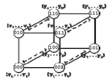
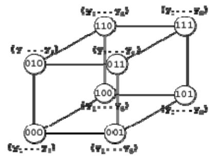
Figure 5. Interprocessor communications on 3D-hypercube (Source: Tanjung, 2002)

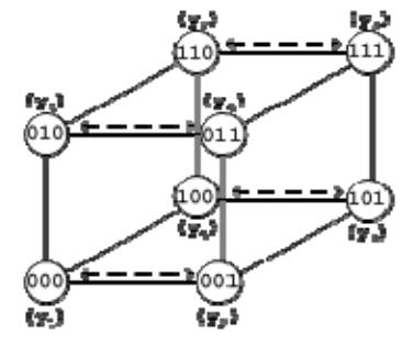
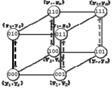
essors. By this way, all processors for analyzing the subdomains of the FEM analysis are only communicating with the processors used to solve the interface problem. Unfortunately, this simple way requires transferring large number of data. This type of interprocessor communication will also reduce the rank of the parallelism since all processors for analyzing the subdomains will idle during solving the interface problem. To improve the simple interprocessor communication above, an interprocessor communication based on the hypercube networking was constructed in this study (Kawamura and Tanjung, 2000, Tanjung, 2002, Kawamura and Tanjung, 2001).

To make clear an understanding of current the interprocessor communication pattern, consider a threedimensional hypercube scheme shown in Figure 5 below for instance.

For the first step, maps the subdomains onto the hypercube networking such that each processor is assigned into different active processor. Then, the interprocessor communication is carried out as graphically shown in the Figure 5. For example, assume that each vector yk in parentheses in the figure denotes the messages, which is required to exchange from one processor to the others. The interprocessor communication starts from the lowest dimension of the hypercube and then proceeds along successively higher dimensions. The processors communicate in pairs with least significant bit of their binary representations. At the termination of communication procedures, each processor will hold the same overall summation result of the vector. Noting that, in the hypercube pattern each processor is only communicate with the neighbours. The neighbours are mapped to hypercube processors whose processor labels differ in exactly one bit position.

Although the CG algorithm requires the interprocessor communication, the algorithm is still amenable to work in the parallel manner. Consider the matrixvector as an example. Each processor evaluates the contribu -

Then exchange the values of the vector yk follows the proposed interprocessor communication pattern mentioned in the foregoing paragraph to obtain the global values containing the contribution from all subdomains. This example clearly shows the attractive CG

algorithm using the communication pattern mentioned above to solve the interface problem (42).

5. Conclusions

Comparing the proposed interprocessor communication pattern based on the hypercube with the simple communication ones, the advantages of the proposed pattern are clearly shown. Each processor is only needed to exchange data in the vector type instead of the matrix/vector in the simple communication pattern. The proposed communication pattern also does not require an additional processor to perform stand alone the CG algorithm. Finally, all of active processors almost never idle since the computation still is conducted in parallel manner even for conducting the CG algorithms.