
Abstrak
Penurunan penggunaan angkutan umum dan peningkatan ketergantungan pada pemakaian kendaraan pribadi telah dialami oleh banyak kota di dunia. Akibat negatifnya terhadap lingkungan sangat mengkhawatirkan. Untuk mencapai kota yang berkelanjutan, salah satu targetnya adalah dengan meningkatkan penggunaan angkutan umum dan mengurangi kendaraan-kilometer. Untuk itu sangat penting untuk mengkaji perilaku komuter. Dengan menggunakan Sensus Perjalanan ke Tempat Kerja di Kota Sydney (Australia), paper ini difokuskan untuk menganalisis preferensi komuter dalam melakukan perjalanan dengan bis. Dua metode diaplikasikan yaitu fungsi keinginan dan statistik spasial Moran I. Fungsi keinginan dipergunakan untuk mengukur perilaku komuter yang menggunakan bis, sedangkan statistik spasial Moran I dipergunakan untuk mengkaji keterkaitan spasial atau interaksi antar zona serta untuk menguji signifikansinya secara statistik. Hasil penelitian memperlihatkan bahwa perilaku komuter dari para pekerja tidak stabil secara spasial. Hal ini menunjukkan bahwa penggunaan satu parameter global untuk memperkirakan perjalanan di masa mendatang tidaklah tepat. Perubahan preferensi komuter dengan bis kearah memaksimalkan jarak telah mengakibatkan peningkatan jarak perjalanan dan kendaraan-kilometer. Statistik spasial memperlihatkan bahwa terjadi interaksi positif untuk perjalanan kerja dengan menggunakan bus.
Kata-kata Kunci: Preferensi komuter, bis, keterkaitan spasial.
1. Introduction
In urban areas, increased sprawl and automobile dependence has been criticized as having a negative impact on transportation efficiency and environmental quality. OECD (1996) stated that these patterns of automobile dependence are not sustainable from both economical and environmental perspective. The negative effects of traffic include lost time and productivity, vehicular accidents, greenhouse gas emissions, deteriorating air quality and associated risks on respiratory and cardiovascular health, among others (Dahl, 2005; WHO, 2005). Such problems are more acute in the US and Australia where low-density and sprawling development pattern to the outer area has increased car dependence (Newman and Kenworthy, 1999). Policies for sustainable urban development should therefore include measures to reduce the need for movement and to provide favorable conditions for energy-efficient and environmentally friendly forms of transport such as bus. Understanding the commuting behavior as a result of urban form changes over time is the interest of this study.
The reduction in vehicle kilometer traveled (VKT) is one of the policy objectives adopted by many cities in order to achieve environmentally sustainable transportation (OECD, 1996; Newman and Kenworthy, 1999; Black, et.al., 2001). Improving the quality of urban public transport is one of many strategies proposed to improve mobility options for the transport disadvantaged (BIC, 2003) and to address car dependence and the urban congestion, environmental sustainability and global warming concerns associated with car dependence (Hamilton, 2006). Improving bus-based public transport has been considered a more costeffective option compared to rail investment (US General Accounting Office, 2001; UK Commission for Integrated Transport, 2005) particularly in relation to the lower density environments associated with Australian and North American cities (Fleming, et.al, 2001; Currie, 2006).
However, according to Holmgren et.al (2008), local public transport development in Sweden, like in many other European countries, has for a long time been on the decline. A similar pattern is found in Great Britain. According to Balcombe et.al (2004) local bus transport has been halved between 1970 and 2000. Mulley and Nelson (2009) stated that an ideal world public transport would be as convenient as private transport, suggesting that 'all public transport should be demand responsive.' Therefore, it is important to understand factors influencing commuting preferences by public transport. Although there is a large amount of research on factors influencing commuting behavior (VanVugt et.al, 1996; Desalvo and Huq, 1996; Joireman et.al, 1997; Bamberg and Schmidt, 1998) we know very little about how it has changed over time.
Historical analyses of the changing nature of the commuting preferences by public transport are relatively rare and concentrate mainly on alterations in the relationship between home and workplace, and the changing structure of the city. Historical study of the journey to work in Toronto during 1900-40 suggests that the decentralization of employment opportunities tended to shorten the journey to work for men, who lived in suburban locations, but disadvantaged women who continued to work mainly in down-town locations (Harris and Bloomfield, 1997). In another study, Pooley and Turnbull (2000) used 1834 individual life histories to examine changes in journey to work transport modes in Britain since 1890 and 1990 in-depth interviews to investigate modal choice amongst commuters since the 1930s. They found that there have been three main periods of change in the transport mode used for commuting, but there has also been considerable inertia in individual modal choice.
The journey to work is one of the most commonly experienced forms of every-day travel, encompassing almost all transport modes, and making a substantial contribution to urban traffic congestion (Pooley and Turnbull, 2000). The weakness in most of the journeyto-work trip studies was the use of a static approach (i.e. the analysis was done at one point in time) (Black, et.al, 2002). It is essential to understand how commuting behavior contributes to either longer or shorter journeys. One way of doing this is to examine the commuting preferences of residents, and to establish how they have changed over time since the redistribution of employment and residential workers. Preference functions can be used to evaluate the behavioral response change of the residents following the change in urban form over time at the zonal level (Black et.al, 2002; Black and Suthanaya, 2002).
The objectives of this study are: to analyze the stability of commuting distance preferences by all transportation modes and by bus of the Sydney's residents and to analyze spatial association of the slope preference functions among zones.
2. Literature Review
2.1 Theory of preference functions
Preference function is an aggregate of individual travel behavioral responses by a zonal grouping given a particular opportunity surface distribution of activities surrounding those travelers. Operationally, a journey-to-work preference function is the relationship between the proportion of travelers from a designated origin zone who reach their workplace destination zones, given that they have passed a certain proportion of the total metropolitan jobs. To derive such functions information is contained in O-D matrices. Proportion of zonal totals and metropolitan totals are used for standardization purposes, rather than absolute numbers, to facilitate comparison of the shape of preference functions across origin zones within a city, across different cities, and within the same city over time. Conceptually, the raw preference function is simply the inverse of Stouffer's intervening opportunity theory (Stouffer, 1940) that relates the proportion of migrants (travelers) continuing given reaching various proportion of the opportunities reached – or more technically-correct the l-factor parameter in the intervening opportunities model of trip distribution (Ruiter, 1969). Stouffer's hypothesis formed the basis of operational models of trip distribution in some early land-use and transportation studies in the United States of America (for example, the Chicago Area Transportation Study during the late 1950s), and is expressed as:
\[P(dv) = (1-P(v) f(v))dv\] (1)
Where:...
where
P(dv) : probability of locating within the dv oppor tunities, P(dv) = dP;
P(v) : probability of having found a location within the v opportunities;
1-P(v) : probability of not having found a locationwithin the v opportunities; and f(v).dv : probability density function of finding a suitable location within the dv opportuneties given that a suitable location has not already been found.
The term f(v) is often called the l parameter, or calibration parameter. It is the ordinate of a probability density function for finding a suitable location given that a location has not already been found. So, Equation (1) may be rewritten as:
\[dP = (1-P). l. dv\] (2)
If l is a constant and the initial conditions are P=0 when v=0 then:
\[lv = -Ln(1-P)\] (3)
Hence,
\[P = 1 - e^{-lv} \tag{4}\]
Whereas Equation (4) is used to derive trip distribution models, Equation (3) is the mathematical expression for the preference function. The relationship between the cumulative total number of opportunities passed, v, and the natural logarithm of the cumulative total number of opportunities taken, Ln (1-P), is assumed to be linear. One of the issues was calibrating the l-factor parameter (Ruiter, 1969), and whether there was a break of slope to justify different parameters for "short" and "long" trips.
The logarithmic curve of the preference function might be linearized using natural logarithmic transformation. The shifting trend of the preference function can then be evaluated by analyzing the change in the slope of preference instead of using visual inspection on the superimposed curves. This is in line with the theory of the intervening opportunities model, where it is stated that the preference functions should have linear form in which Xi,t being transformed to -Ln (Xi, t). The shape of the observed preference functions is transformed as follows using regression analysis:
\[Y = a \left[ -\ln (X) \right] + b \tag{5}\] where:
Y = cumulative proportion of zonal metropolitan jobs taken from each origin zone;
X = cumulative proportion of zonal jobs reached from each origin zone;
a = regression coefficient;
b = regression constant.
Unlike the raw preference functions these are the transformed preference functions with negative gradients, as in the above formula, where small (absolute) values of parameter a are associated with a preference for shorter trips and large (absolute) values are associated with a preference for longer trips, everything else being equal. The slope of these empirically determined preference functions tells us much about travel behavior as a pure response to opportunities, and not to transport impedance (distance, time or cost) as in the gravity model of trip distribution.
2.2 Spatial statistics
To test the hypothesis of spatial stability, which implies that the preference function is similar across all geographical units, Moran's I statistic of spatial association is used. There are qualitative differences among zones in terms of the preference function gradient, but a more rigorous test is required to discard the possibility that variation is random. A statistic of spatial autocorrelation, such as Moran's I (Moran, 1948; Cliff and Ord, 1969), provides the tool to test this hypothesis. Spatial association is a measure of a variable's correlation in reference to its spatial location. In the case of Moran's I, the measure is that of covariance between variable values at locations sharing some sort of common boundary or connection. In general, when values are interrelated in meaningful spatial patterns it is said that there is spatial association. The statistic then measures the strength of the relationship, and its general quality. When similar values (in deviations from the mean) are found at neighboring locations, positive spatial autocorrelation results. When dissimilar values are found at neighboring locations, negative spatial association is said to ensue. Zero association is obtained when there are no significant similarities, or dissimilarities, amongst values, as would be the case for instance of a very homogeneous set of observations. Spatial association is computed by:
- 1. Assigning weights to the cases, based on number of trips in a (square) O-D matrix and the transpose D-O matrix;
- 2. Row-standardizing the matrix to obtain zonal trip proportions (so that the sum of proportions equals 1 in each row), to facilitate the comparison across zones to allow us to test for spatial stability.
The result is a connectivity matrix W that defines the 'neighborhood' (the zones with which there is interaction) for each zone. When using row-standardized connectivity matrices, computation of Moran's I is achieved by division of the spatial co-variation by the total variation:
\[I = \frac{\sum \sum w_{ij} (x_i - \overline{x})(x_j - \overline{x})}{(x_i - \overline{x})^2} = \frac{\sum \sum w_{ij} \hat{x}_i \hat{x}_j}{\hat{x}_i^2} \quad i \neq j\] (6)
where
= the mean of the observations \(\overline{x}\)
\(w_{ij}\) = the proportion of trips between i and j, with respect to the total from i.
If the value of I is positive, this represents positive spatial autocorrelation; if negative it represents negative spatial autocorrelation. A zero value of I represents random variation, and thus no spatial autocorrelation. Inference can be carried out by comparing it to its expected value and variance, to obtain a normalized statistic Z (I), since the statistic is asymptotically normally distributed (for technical details see Cliff and Ord, 1969). A useful characteristic of the above statistic, more easily seen if represented in matrix notation, is its formal resemblance to a regression of the spatially lagged variable on variable:
\[I = \frac{\hat{\mathbf{x}}' \mathbf{W} \hat{\mathbf{x}}}{\hat{\mathbf{x}}' \hat{\mathbf{x}}} = (\hat{\mathbf{x}}' \hat{\mathbf{x}})^{-1} \hat{\mathbf{x}}' \mathbf{W} \hat{\mathbf{x}}\](7)
I is interpreted as the slope of a line passing through the origin. This decomposition into two variables, with one spatially lagged, can be illustrated as a scatter-plot to obtain a Moran's Scatter-plot (Anselin, 1995).
3. Methodology
3.1 Study area and data sources
Sydney Metropolitan Region is selected as a case study area with the population reached 4 million. The population in the outer suburbs has increased at a much faster rate than that in the inner and middle ring suburbs. The configuration of the 44 LGAs is shown in Figure 1. This analysis uses time-series journey-towork (JTW) census data over a 35 years period from 1961 to 1996 for the analyses of preference function by all transportation modes. In these data sets, the traffic zones are aggregated into 38 LGAs to provide a consistent number of LGAs over time from 1961 to 1996. However, for the analyses of preference function by bus, the JTW census data sets available are for the 1981, 1991 and 1996 period. Inter-zonal (LGA) distances over the road network were provided by the NSW State Transport Study Group, now the Transport Data Centre.
3.2 Analytical method
Journey-to-work (JTW) census data and impedance matrix data are used as input. From these data, origindestination (O-D) matrices by local government area (LGA) are developed for all transportation modes and also, separately for bus. Preference function is applied
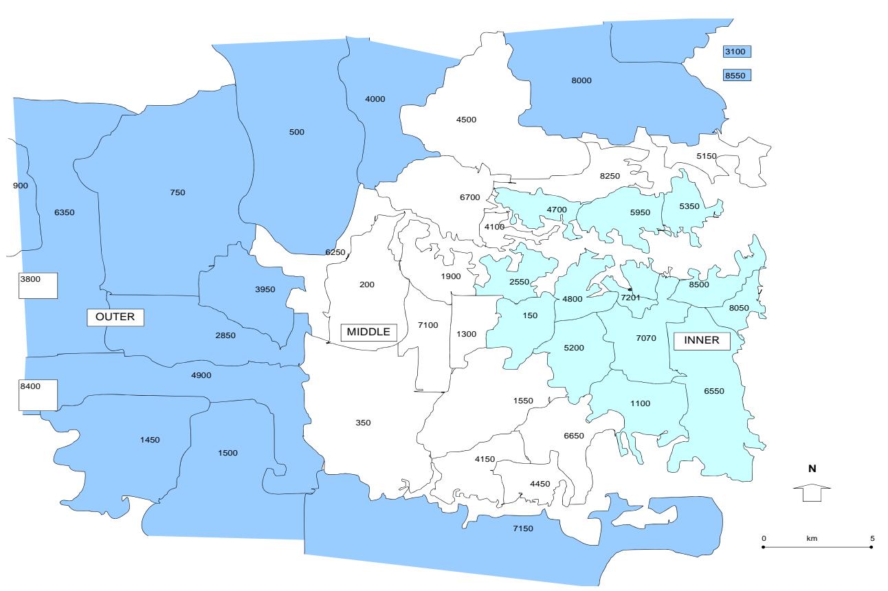
Figure 1. Sydney zoning system Source: NSW Transport data centre (2002)
to study the journey-to-work commuting preferences. Destination zones are ranked based on the impedance matrix data - centroid to centroid zonal distance. Cumulative proportion of jobs reached and cumulative proportion of zonal (LGA) trips are then calculated followed by curve fitting of the preference function. For evaluation and comparison purposes, the curve is transformed into linear form. The slope preferences obtained from this transformation are used for an evaluation of shifting trends and zone performance. Descriptive statistics and analysis of variance are applied to evaluate the trends in the slope preferences over time. Moran's I statistic of spatial association is used to study the spatial distribution of preference functions, and the pattern of interactions between zones, to assess the level of interaction and to test their statistical significance. Moran's scatter-plot is used for visual inspection and detecting outliers. The results are then used to interpret the policy implication of the commuting behavior stability in Sydney.
4. Results and Discussions
4.1 Commuting preferences by all transportation modes
Figure 2 shows that the mean slope (absolute value) of preference functions by all transportation modes for 38 LGAs in Sydney increased very slightly during 1961- 1976 period from 0.197 in 1961 to 0.199 in 1976 and was then followed by a slightly steeper increase reaching 0.210 in 1996. The slope will likely continue to increase slightly in the future if the distribution of residential workers and jobs and travel behavior follows existing trends. Continuation of decentralization trends in a scattered form will lead the behavioral preferences of residents toward longer trips or towards the distance maximization upperbound. When plotted by the LGA's
location at increasing distances from the CBD, Figure 3 shows that several LGAs in the inner and middle ring experience little change in the absolute value of the slope preferences during the 35 years period from 1961 to 1996. The slopes are relatively stable in these areas. On the other hand, there is an increase in the slope (in absolute terms) experienced by the LGAs in the outer ring (beyond 20 km from the CBD). Despite decentralization of employment towards the outer areas experienced in Sydney during this period, the scattered location of the development may explain the change in the behavioral response of residents towards longer trip, or maximizing distance behavior. This indicates that in order to stabilize or slow the growth of resident preferences for longer trips in the outer areas, distribution of employment needs to be shaped and focused in several key areas instead of scattered evenly across the outer ring LGAs.
4.2 Commuting preferences by bus
By increasing LGA distances from the CBD, Figure 4 shows that the absolute value of the slope preferences by bus tend to decrease. This indicates that LGAs located further away from the CBD have preferences towards shorter trips to work by bus. Residents in the outer ring tend to use bus for local or short distance commuting trips only. On average in the outer ring, the slope preference by bus has increased by about 0.091 per 5 years from 0.022 in 1981 to 0.296 in 1996. On the other hand, residents in the inner ring tend to use bus for traveling to work for longer distance commuter trips. Unlike car, the slope preferences by bus are relatively more stable over time regardless of the LGA distance from the CBD. However, several extreme cases were identified. A substantial increase in the absolute value of the slope preferences by bus is experienced in the Sydney LGA (about 0.145 per 5 years
Slope by All Transportation Modes
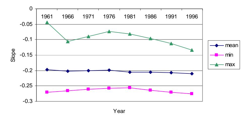
Figure 2. The mean slope preferences for 38 LGAs in Sydney (1961-1996) Source: NSW Transport data centre (2002); Analysis results (2010)
from 0.240 in 1981 to 0.676 in 1996). South Sydney, located in the inner ring, also experienced a high increase although at a lesser rate (about 0.035 per 5 years from 0.250 in 1981 to 0.354 in 1996).
Furthermore, Table 1 summaries descriptive statistics of the slope preferences by bus in Sydney over a 15 year period from 1981 to 1996. The descriptive statistics reveal that the absolute value of the slope preferences by bus has increased by about 0.024 over the period from 0.150 in 1981 to 0.174 in 1996. This indicates that the behavioral preference of residents for commuting by bus has moved toward longer trips or distance maximizing trends. The lowest value of the slope in absolute terms increased constantly from 0.009 in 1981 to 0.028 in 1996 whilst the highest absolute value of the slope increased at a steeper rate from 0.292 in 1981 to 0.676 in 1996.
4.3 Spatial analysis of the commuting preferences by bus
To test the hypothesis of spatial stability of the distribution of slope preference, Moran's I is applied. Moran's scatter-plot based on Anselin (1995) is also applied to visually inspect the spatial interaction of the slope preferences between zones. Figure 5 shows the Moran's scatter-plot for the distribution of zonal slope preferences by bus in Sydney in 1996. The variation of zonal slope preferences by bus is not very extreme as most of the slope preferences are within one standard deviation and only a few zones are beyond one standard deviation on either the minimization or the maximization side. However, one extreme case was identified where Sydney (38) has slope preferences beyond four standard deviations on the maximization side. Moran's statistic of I = 1.250, indicates the existence of positive spatial autocorrelation. Further significance testing with Z-statistic, Z(I) = 10.39 indicates the significance of this positive spatial autocorrelation. The residents in the zones with high slope (preferences towards longer trips) tend to interact with zones having high values (absolute) of slope preferences. On the other hand, the residents in zones with low absolute slope preferences tend to travel to zones also with low absolute slope or zones with preferences towards distance minimization.
Scatter-plot of the average change in the slope preferences by bus per 5 year shown at the bottom of Figure 5 indicates that the values are mainly within one standard deviation from the mean. Only one extreme case was identified where Sydney (38) experienced an increase in the slope preference by bus of
Table 1. Summary of descriptive statistics of the slope preferences by Bus in Sydney (1981-1996)
| Statistics | 1981 | 1991 | 1996 |
|---|---|---|---|
| Mean | -0.150 | -0.160 | -0.169 |
| Standard deviation | 0.089 | 0.101 | 0.120 |
| Minimum | -0.292 | -0.470 | -0.676 |
| Maximum | -0.009 | -0.025 | -0.028 |
| Range | 0.283 | 0.446 | 0.647 |
Source: Analysis results (2009)
Slope Preference and Distance from CBD
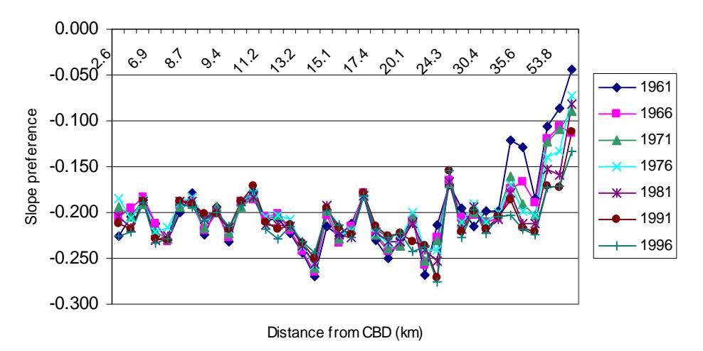
Figure 3. Slope preference functions by increasing distance from CBD (1961-1996) Source: NSW Transport data centre (2002); Analysis results (2009)
Bus Slope and Distance from CBD
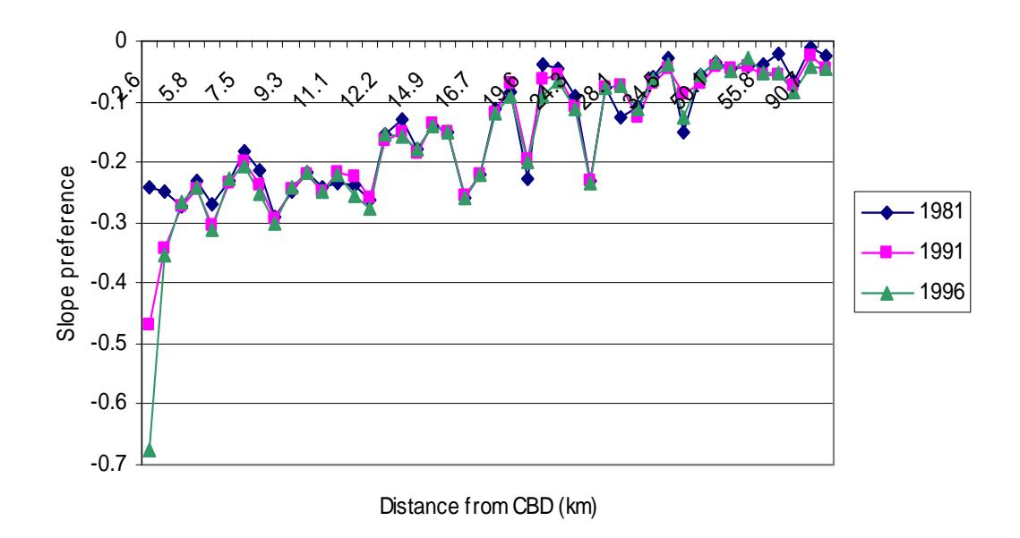
Figure 4. Slope preference by bus in Sydney by increasing LGA distance from the CBD Source: Analysis results (2009)
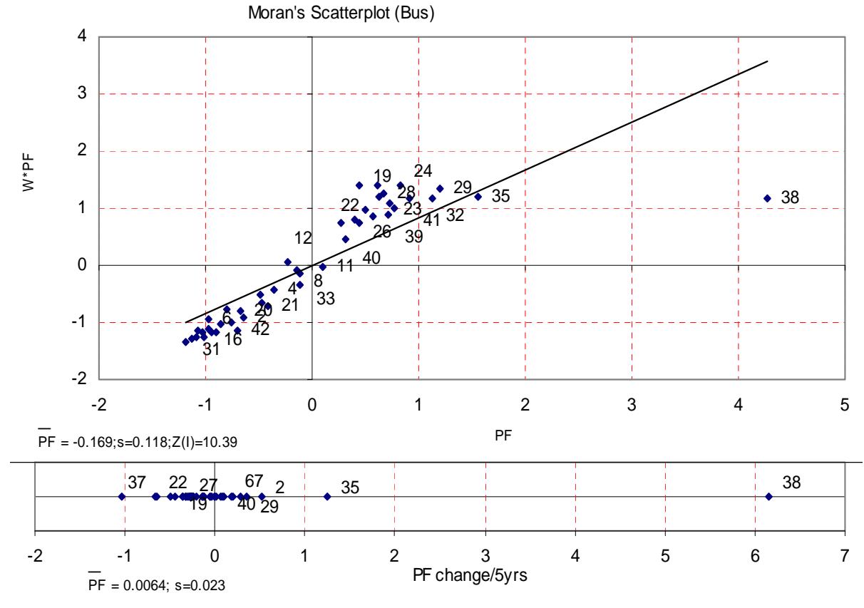
Figure 5. Moran's Scatter-plot for slope preferences by bus (1996) Source: Analysis results (2009)
over six standard deviations above the mean value. This indicates an increasing preference of residents in Sydney LGA to use bus for traveling to work for longer distances over time given already having a high absolute value
Figure 6 explains further that an extensive bus service in the inner areas (within 11 km from the CBD), enable people living in the inner ring to travel longer by bus to reach their work place, in particular, to the CBD destination (for example in the figure, Sydney (38) and Leichardt (24)). Residents living in Sydney (38) tend to travel longer by bus to reach their work place given the high intensity of bus services in this LGA. People living in Penrith (31) tend to take the bus mainly for local and relatively short trips, whilst car dominates long distance trips. The proportion of workers using bus in the outer areas is much lower than that in the inner and middle areas because of the lack of reliable bus services. Low density and scattered jobs locations make it much more convenient for these outer ring residents to travel by car.
By considering the destination-origin (D-O) matrix, a positive spatial association is also experienced as shown in Moran's scatter-plot (Figure Zones with preference towards distance maximization tend to attract trips from zones which also show maximization preferences. On the other hand, zones with preference towards distance minimization tend to attract trips from zones with similar preferences.
Proportion Working by Bus Vs Distance from CBD
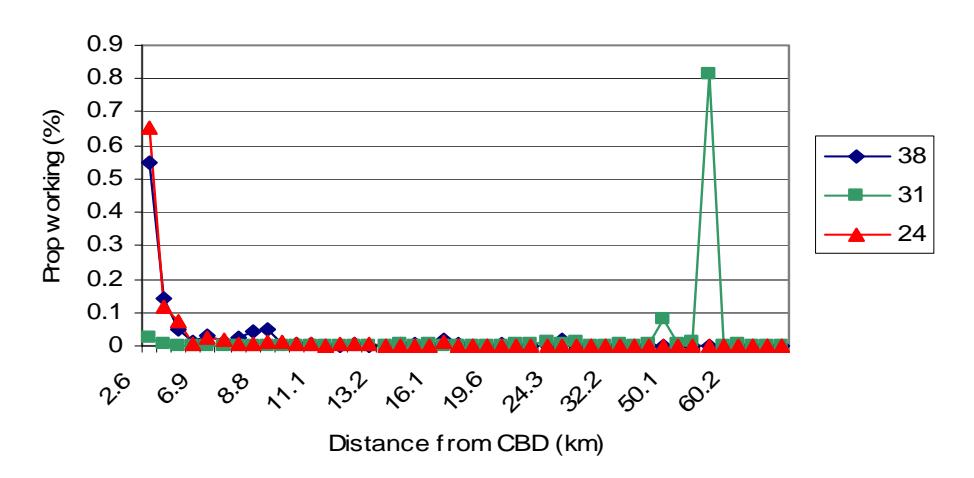
Figure 6. Proportion of residents working by bus by increasing distance from the CBD Source: Analysis results (2009)
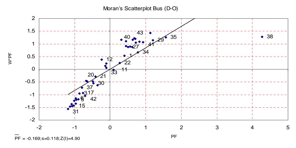
Figure 7. Moran's scatter-plot for slope preferences by bus (1996) using D-O matrix Source: Analysis results (2009)
This positive spatial association is confirmed further from Moran's I statistic with I = 0.589 and Z(I) = 4.90.
5. Conclusions
Based on the results of commuting preference and spatial autocorrelation analyses, the following conclusions were withdrawn:
- 1. In general, the increase of the mean slope preference over time indicated the increasing preference for residents to travel for longer distances over time. However, the outer ring residents tended to use bus for shorter distance trips compared to that in the inner and middle ring residents.
- 2. The slope preferences were mostly stable in the inner and middle ring whilst substantial increase was experienced by LGAs in the outer ring (beyond 20 km from the CBD). Therefore, in order to stabilize or slow the growth of resident preferences for longer trips in the outer areas, distribution of employment needs to be shaped and focused in several key areas instead of scattered evenly across the outer ring LGAs.
- 3. A significant positive spatial association was identified for the slope preferences by bus for both O-D and D-O matrices. Zones with preference towards distance maximization tended to attract trips from zones which also show maximization preferences. On the other hand, zones with preference towards distance minimization tended to attract trips from zones with similar preferences.
6. Acknowledgements
The author would like to express his gratitude and appreciation to Professor John Black, the University of New South Wales, Sydney, Australia for his great support and to NSW Transport Data Centre for providing data.