
Abstract
Telah diketahui bahwa perilaku tanah akan tergantung dari sejarah pembebanannya dan juga memperlihatkan perilaku hardening apabila tanah mengalami deformasi secara plastik. Tulisan ini menyajikan sebuah formulasi model tanah mixed hardening multisurface hyperplasticity dengan faktor kekakuan kinematik hardening proporsional terhadap tekanan pra-konsolidasi guna merepresentasikan sejarah pembebanan yang terjadi pada tanah. Formulasi ditekankan untuk mendeskripsikan perilaku pembebanan siklik pada tanah lempung. Kelebihan dari pendekatan model hyperplasticity ini adalah dapat menghasilkan transisi dari perilaku elastik ke plastik secara smooth serta mampu "mengingat" sejarah perubahan tegangan yang terjadi pada tanah dengan menggunakan fungsi variabel internal. Fungsi leleh Modified Cam Clay dipilih sebagai model utama untuk mensimulasikan respons tegangan-regangan. Selanjutnya, respons tegangan-regangan dihitung berdasarkan sebuah formulasi rate-dependent. Terakhir, tulisan ini mendeskripsikan pentingnya pengembangan model ini guna memperbaiki analisis respons tanah akibat gempa. Hasil-hasil lebih lanjut berupa implementasi dan simulasi numerik serta juga verifikasi model yang diusulkan akan disajikan dalam publikasi berikutnya.
Kata-kata Kunci: Hyperplasticity, mixed hardening, tekanan pra-konsolidasi, analisis respons tanah akibat gempa.
1. Introduction
In modeling geomaterials, it is clear that multisurface models are able to fit the non-linear behavior more accurately across a wide range of strain amplitude. Within the framework of "continuous hyperplasticity", it is also possible to generalize a multisurface model into an infinite number of yield surfaces.
Further, it is well-known that soil behavior is dependent upon the history of loading and exhibits hardening behavior when deformed plastically. In the early developments of critical state soil models (Roscoe and Burland, 1968); Schofield and Wroth, 1968) the history of loading that represented by pre-consolidation pressure is taken as a function of the void ratio to describe the size of the yield surface during unloadingreloading cycles. As for the size of the yield surface, another more recent suggestion that is valid from both dimensional and thermo-mechanical considerations (Hashiguchi, 1974; Butterfield, 1979; Collins and Kelly, 2002) is to take the pre-consolidation pressure as a function of the plastic volumetric strain rather than the void ratio. Moreover, various cyclic constitutive models have been proposed to date which can be classified into three classes: equivalent linear models (Schnabel et al., 1972; Bardet et al., 2000), cyclic nonlinear models (Streeter et al., 1973; Joyner et al., 1977; Lee and Finn, 1978; Martin and Seed, 1978; and Pyke, 1985) and advanced constitutive models based on the idea of isotropic hardening (Hashiguchi and Ueno, 1977; Hashiguchi, 1989) and kinematic hardening (Mroz, 1967; Iwan, 1967; Dafalias and Popov, 1975; Prevost, 1989; Bardet and Tobita, 2001) for evaluating the effects of local soil conditions on ground response during earthquakes.
Apriadi (2009a) and Apriadi et. al. (2009b) employed a non-linear continuous hyperplasticty kinematic hardening MCC model by extending the work of Likitlersuang (Likitlersuang, 2003; Likitlersuang & Houlsby, 2006). In this model, the stiffness factors of the kinematic hardening of the yield surfaces proportional to the current pressure. Several model features of this model for describing cyclic behavior of soils such as irreversible unloading-reloading response, a hysteresis loop with accumulation shear strain and smooth transition of stiffness during unloading-reloading cycles have been presented. It is clearly shown that the dominant hardening processes such that the Bauschinger effect can be represented very well. Moreover, the developed model can also describe a non -linear behavior of soils more accurately across a wide range of strain amplitude. However, over (normally) quite large numbers of cycles the soils exhibit a combined isotropic and kinematic hardening or mixed hardening behavior (Dunne and Petrinic, 2005).
The objective of this work is to formulate a mixed hardening multisurface hyperplasticity model with stiffness factors of the kinematic hardening of the yield surfaces proportional to the pre-consolidation pressure rather than the current pressure. We initially describe some definitions of pre-consolidation pressure and continue with a formulation of the model in general stress conditions rather than triaxial stress conditions, followed by an explanation of the recent constitutive modeling in ground response analysis. Finally remarks are made on the features of the proposed model. This study is expected to contribute for improvement of load-deformation prediction in earthquake ground response analysis.
2. Pre-consolidation Pressure in Stress Space
In critical state soil mechanics, the pre-consolidation pressure describes the asymptotic behavior of the model under isotropic (q = 0) normal compression conditions \((p = p_c)\) using some kinematic variables as shown in Figure 1.
In the original critical state models Roscoe and Burland (1968); and Schofield and Wroth (1968) proposed the expression for the pre-consolidation pressure by:
\[P_c = P_r \exp\left(\frac{v_{\lambda} - v}{\lambda}\right) \tag{1}\] where \(p_r\) is a reference pressure, \(v_l\) is specific volume at the reference pressure and \(\lambda\) is slope of normal compression line in v: log p. The pre-consolidation pressure was expressed purely using the specific volume v = 1+e (with e being the void ratio). In this model the void ratio related to the logarithm of the pressure and the size of yield surface is expressed using the void ratio as shown in Figure 2.
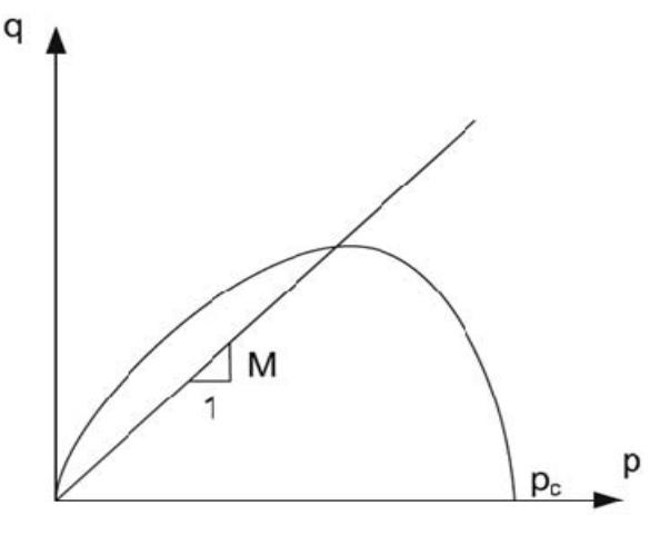
Figure 1. Definition of pre-consolidation pressure in typical yield surface projection in stress-space (Einav and Carter, 2007)
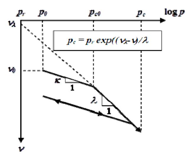
Figure 2. Original definition of pre-consolidation pressure (Einav and Carter, 2007)
Another more recent suggestion, which is based from both dimensional and thermo-mechanical considerations (Hashiguchi, 1974; Butterfield, 1979; Collins and Kelly, 2002) is to express linearity between the preconsolidation pressure and the void ratio in log-log space, i.e., a linear relation between \(\log(p_c)\) and \(\log(v)\), also the size of yield surface is expressed using the preconsolidation pressure as shown in Figure 3.
In this definition, the expression for the preconsolidation pressure is expressed using plastic volumetric strain \(e_v^p\) by:
\[P_c = P_{c0} \exp\left(\frac{\varepsilon_v^p}{\lambda^* - \kappa^*}\right) \tag{2}\] where \(P_{c\theta}\) is initial pre-consolidation pressure, \(\lambda^*\) is slope of normal compression line in log \((\nu)\): log (p) and \(k^*\) is slope of unloading-reloading line in log \((\nu)\): log (p).
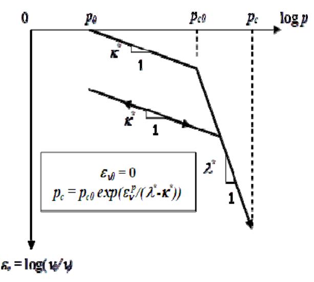
Figure 3. Linearity between the pre-consolidation pressure and the void ratio in log-log space (Einav and Carter, 2007)
Two definitions in Equation (1) and Equation (2) are quite significant. In the first definition, the specific volume at the reference pressure, \(v_{\lambda}\) is defined as the reference kinematic configuration which is unique for a given soil while in the second definition this parameter is represented by the initial pre-consolidation pressure, \(p_{c0}\) which is dependent upon the history of loading.
3. Mixed Hardening Modified Cam Clay Model
3.1 Sign convention
The standard soil mechanics sign convention of compressive stresses and strains positive is used throughout this paper, and all stresses are effective. The following notation is adopted: \(\sigma_{ij}\) is the effective Cauchy stress tensor; \(\varepsilon_{ij}\) is small-strain tensor; and \(\delta_{ij}\) is Kronecker's delta (\(\delta_{ij} = 1\) if i = j, \(\delta_{ij} = 0\) if \(i \neq j\) where i, j \(\hat{I}\) {1,2,3}).
The stress invariants are \(p = \frac{1}{3}\sigma_{ii}\) , \(q = \sqrt{\frac{3}{2}\sigma'_{ij}\sigma'_{ij}}\)
where \[\sigma_{ii} = \sum_{k=1}^{3} \sigma_{kk}\] , \(\sigma'_{ij} = \sigma_{ij} - p\delta_{ij}\) is deviatoric
component of the effective stress tensor. The corresponding strain invariants are
\[\varepsilon_p = \varepsilon_{ii}\] and \(\varepsilon_q = \sqrt{\frac{2}{3} \varepsilon'_{ij} \varepsilon'_{ij}}\), where \(\varepsilon'_{ij} = \varepsilon_{ij} - \frac{1}{3} \varepsilon_{ii} \delta_{ij}\)
is a deviatoric component of the strain tensor. Similarly, generalized stress invariants are
\[\chi_p = \frac{1}{3} \chi_{ii}\], \(\chi_q = \sqrt{\frac{3}{2} \chi'_{ij} \chi'_{ij}}\) where \(\chi_{ii} = \sum_{k=1}^{3} \chi_{kk}\)
\(\chi'_{ii} = \chi_{ii} - \chi_p \delta_{ii}\)
is a deviatoric component of the effective generalised stress tensor. The corresponding internal variable invariants are
\[\alpha_p = \alpha_{ii}\] and \(\alpha_q = \sqrt{\frac{2}{3}\alpha'_{ii}\alpha'_{ii}}\) where \(\alpha'_{ii} = \alpha_{ii} - \frac{1}{3}\alpha_{ii}\delta_{ii}\)
is deviatoric component of the internal variable tensor.
3.2 Model formulation
Under the hyperplasticity framework (Houlsby and Puzrin, 2006), a non-linear continuous hyperplasticity mixed hardening Modified Cam Clay (MCC) model is formulated to the Gibbs free energy by considering pre-consolidation pressure dependency in Equation (2) and non-linear elastic moduli at small-strain (Houlsby et al., 2005):
\[E = -\frac{p_e^{2-n}}{p_r^{1-n}k(1-n)(2-n)} + \frac{\sigma_{kk}}{3k(1-n)} - \sigma_{ij}\alpha_{ij} + \frac{1}{9} \left( \frac{\hat{H}_p \hat{\alpha}_{kk}^2}{2} + \frac{\hat{H}_q \hat{\alpha}_{ij}^{\prime} \hat{\alpha}_{ij}^{\prime}}{3} \right) d\eta + (\lambda^* - \kappa^*) P_{c0} \exp\left( \frac{\alpha_{kk}}{\lambda^* - \kappa^*} \right)\](3)
where
\[p_e = \sqrt{\frac{\sigma_{ii}\sigma_{jj}}{9} + \frac{k(1-n)\sigma'_{ij}\sigma'_{ij}}{2g}}\] is defined as an equivalent
stress variable for convenience.
k, g, and n are dimensionless material constant calibrated from elastic stress-strain relation at small-strain level. Atmospheric pressure 1 atm (approximately 100 kPa) is defined for \(p_r\) as a reference pressure. \(P_{c0} = \sigma_{c0kk}/3\) is an initial pre-consolidation pressure, \(\lambda^*\) is slope of normal compression line in log (\(\nu\)): log (p) and \(k^*\) is slope of unloading-reloading line in log (\(\nu\)): log (p). \(a_{ij}\) is total plastic strain tensor. Integration of differential hardening energy is evaluated in terms of internal coordinate n which is in range of 0 to 1.
\(\hat{\alpha}_{ij}\) is kinematic internal variable tensor function of \(\eta\)
which can be integrated to obtain \(\alpha_{ij}\) using Equation (4). It is important noted that all variables with "\(\text{[rumus tidak dapat ditampilkan dengan baik — lihat PDF asli]}\)
\[\alpha_{ij} = \int_{0}^{1} \hat{\alpha}_{ij} d\eta \tag{4}\]
\(\hat{H}_{n},\hat{H}_{a}\) [in kPa] are non-linear kinematic hardening
functions corresponding to isotropic and deviatoric hardening responses as expressed in Equations (5) and (6).
\[\hat{H}_{p} = \frac{kp_{c0}^{n} p_{r}^{1-n} (1-\eta)^{3}}{2(a-1)}\] (5)
\[\hat{H}_{q} = \frac{3gp_{c0}^{n}p_{r}^{1-n}(1-\eta)^{3}}{2(a-1)}\] (6)
where a is a material hardening constant.
In the hyper plasticity framework, total strain components are considered as conjugate variables of stresses which are derived from the Gibbs energy function. From Equation (3), the strains \(\varepsilon_{ij}\) can be obtained via differentiation with stresses \(\sigma_{ij}\) as shown in Equation (7).
\[\varepsilon_{ij} = -\frac{\partial E}{\partial \sigma_{ij}} = \frac{1}{3k(1-n)} \left[ \frac{\sigma_{kk}}{3p_r^{1-n}p_e^n} - 1 \right] \delta_{ij} + \frac{\sigma'_{ij}}{2gp_r^{1-n}p_e^n} + \alpha_{ij}\] (7)
However, the Gibbs energy function expressed in Equation (3) and the strain components derived in
Equations (7) can only produce a constant modulus (n = 0) or power function of pressure dependent modulus (0 < n < 1). For linear pressure dependent modulus (n = 1) these equations will be replaced by Equations (8) and (9).
\[E = -\frac{\sigma_{ii}}{3k} \left( \ln \left( \frac{\sigma_{ij}}{3p_r} \right) - 1 \right) - \frac{3\sigma'_{ij}\sigma'_{ij}}{4g\sigma_{kk}} - \sigma_{ij}\alpha_{ij} + \int_{0}^{1} \left( \frac{\hat{H}_{p}\hat{\alpha}_{kk}^{2}}{2} + \frac{\hat{H}_{q}\hat{\alpha}'_{ij}\hat{\alpha}'_{ij}}{3} \right) d\eta + \left( \lambda^{*} - \kappa^{*} \right) P_{c0} \exp \left( \frac{\alpha_{kk}}{\lambda^{*} - \kappa^{*}} \right)\] (8)
\[\varepsilon_{ij} = -\frac{\partial E}{\partial \sigma_{ij}} = \left(\frac{1}{3k} \ln \left[\frac{\sigma_{kk}}{3p_r}\right] - \frac{3\sigma'_{ij} \cdot \sigma'_{ij}}{4g\sigma_{ii}\sigma_{jj}}\right) \cdot \delta_{ij} + \frac{\sigma'_{ij}}{2gp_r^{1-n}p_e^n} + \alpha_{ij}\] (9)
The second derivatives of Gibbs free energy are derived in Box 1. This form is applicable to \(0 \le n \le 1\).
Further, the yield function in term of generalized stress variables is defined:
\[\hat{y} = \sqrt{\frac{\hat{\chi}_{kk}^2}{9} + \frac{3}{2} \frac{\hat{\chi}_{ij}' \hat{\chi}_{ij}'}{M^2}} - \hat{c} = 0\] (10)
where M is a frictional critical state parameter (Roscoe and Burland, 1968) which is the value that stress ratio q/p 'attains at critical state,
\[\hat{c} = P_{c0} \exp \left( \frac{\alpha_{kk}}{\lambda^* - \kappa^*} \right) \eta \text{ is a hardening stress which}\] represents the size of yield surface function, and \(\hat{\mathcal{X}}_{ij}\) are generalized stresses. When the stress is inside the yield surface \(\hat{y} < 0\), materials behave elastically, but they behave plastically when the yield surface is active (\(\hat{y} \ge 0\)). From Equation (3), it follows that
\[\hat{\chi}_{ij} = \frac{\partial \hat{E}}{\partial \hat{\alpha}_{ij}} = \sigma_{ij} - \hat{H}_{p} \hat{\alpha}_{kk} \delta_{ij} - \frac{2}{3} \hat{H}_{q} \hat{\alpha}'_{ij} - P_{c0} \exp\left(\frac{\alpha_{kk}}{\lambda^{*} - \kappa^{*}}\right) \delta_{ij}\] \[\tag{11}\]
The evolution rule of kinematic internal variable functions \(\hat{\alpha}_{ij}\) is derived from the derivatives of flow potential w with respect to generalised stress variables (Houlsby and Puzrin, 2006):
\[\dot{\hat{\alpha}}_{ij} = \frac{\partial w}{\partial \hat{\chi}_{ij}} \tag{12}\]
Box 1: Second derivatives of Gibbs free energy
\[-\frac{\partial^{2} E}{\partial \sigma_{ij} \partial \sigma_{kl}} = \frac{1}{p_{r}} \left( \frac{p_{r}}{p_{e}} \right)^{n} \left\{ \left( \frac{1}{k} + \frac{n \sigma'_{ij} \sigma'_{ij}}{2g p_{e}^{2}} \right) \frac{\delta_{ij} \delta_{kl}}{9} - \frac{n \sigma_{mm}}{18g p_{e}^{2}} \left( \sigma'_{ij} \delta_{kl} + \delta_{ij} \sigma'_{kl} \right) + \frac{1}{2g} \left( \delta_{ik} \delta_{jl} - \frac{\delta_{kl} \delta_{ij}}{3} \right) \right\}\] \[-\frac{nk \left( 1 - n \right)}{4g^{2} p_{e}^{2}} \sigma'_{ij} \sigma'_{kl}\] \[-\frac{\partial^{2} E}{\partial \hat{\alpha}_{ij} \partial \sigma_{kl}} = \delta_{ij} \delta_{kl} = \text{ identity matrix}\]
One may associate this kind of evolution rule to the flow rule used in classical plasticity. The flow potential w is defined based on elasto-viscoplastic theory (see for detail Zienkiewicz and Cormeau, 1974) in relation to the yield function \(\hat{v}\) as shown in Equation (13).
\[w = \frac{\left\langle \hat{\mathcal{Y}} \right\rangle^2}{2\mu} = \frac{\left\langle \sqrt{\frac{\hat{\mathcal{X}}_{kk}^2}{9} + \frac{3}{2} \frac{\hat{\mathcal{X}}_{ij}' \hat{\mathcal{X}}_{ij}'}{M^2}} - \hat{c} \right\rangle^2}{2\mu} \tag{13}\] where \(\mu\) is the artificial viscosity coefficient in unit of kPa.s [SI units]. It is imposed on unity for ratedependent calculation (Griffiths, 1980) while the operator ( ) are Macaulay brackets which define
\[\langle \bullet \rangle = \begin{cases} 0; & \bullet < 0 \\ \bullet; & \bullet \ge 0 \end{cases}\]
However, we can actually define \(\mu\) as a true viscosity coefficient to incorporate rate-dependent behaviour of soil such as creep problems.
According to Equations (7) and (9), total strain components are derived as function of \(\sigma_{\iota\varphi}\) and \(\alpha_{\iota\varphi}\). By flow rule, rate of change of total strain components can be written by the following equations.
\[\left\{\dot{\varepsilon}_{ij}\right\} = \left[-\frac{\partial^{2} E}{\partial \sigma_{kl} \partial \sigma_{ij}}\right] \left\{\dot{\sigma}_{kl}\right\} + \int_{0}^{1} \left[-\frac{\partial^{2} E}{\partial \hat{\alpha}_{kl} \partial \sigma_{ij}}\right] \left\{\dot{\hat{\alpha}}_{kl}\right\} d\eta \tag{14}\]
By using Equations (12) and (13), the rate form of stress-strain relationship obtained in Equation (14) can be expressed.
\[\left[ -\frac{\partial^{2} E}{\partial \sigma_{ij} \partial \sigma_{kl}} \right] \left\{ \dot{\sigma}_{kl} \right\} = \left\{ \dot{\varepsilon}_{ij} \right\} - \int_{0}^{1} \left[ -\frac{\partial^{2} E}{\partial \sigma_{ij} \partial \hat{\alpha}_{kl}} \right] \left\{ \frac{\partial w}{\partial \hat{\chi}_{ij}} \right\} d\eta \tag{15}\]
The derivative of flow potential w in Equation (13) is shown in Equation (16).
\[\frac{\partial w}{\partial \hat{\chi}_{ij}} = \frac{\sqrt{\frac{\hat{\chi}_{kk}^{2} + \frac{3}{2} \frac{\hat{\chi}_{ij}^{2} \hat{\chi}_{ij}^{2}}{M^{2}}} - P_{c0} \exp\left(\frac{\alpha_{kk}}{\lambda^{*} - \kappa^{*}}\right) \eta}{\mu} \frac{2}{9} \hat{\chi}_{kk}^{2} \delta_{ij}^{2} + \frac{3}{M^{2}} \hat{\chi}_{ij}^{2}}{2\sqrt{\frac{\hat{\chi}_{kk}^{2} + \frac{3}{2} \frac{\hat{\chi}_{ij}^{2} \hat{\chi}_{ij}^{2}}{M^{2}}}}}{(16)}\]
3.3 Model parameter determination
Compared to non-linear kinematic hardening MCC model (Apriadi et al., 2009), the mixed hardening MCC model has eight number of parameters, consisting of three dimensionless material constant parameters (g, k, and n), three parameters for critical state \((M, l^*, k^*)\), and two kinematic hardening parameter \((a, P_{c0})\). These parameters are obtained through processes of parameter calibration from the experiment results (see Apriadi et al. (2009) for details).
4. Constitutive Modeling in Ground Response Analysis
4.1 Recent cyclic constitutive models
Several methods for evaluating the effects of local soil conditions on ground response during earthquakes are presently available. Most of these methods are based on the assumption that the main responses in a soil deposit are caused by the one-dimensionally upward propagation of shear wave from the underlying bed formation (Schnabel et. al, 1972). Computer program developed for this analysis are generally based on either the solution of the wave equation or on a lumped mass simulation. Some of these programs are based on soil constitutive modeling and use either finite different or finite element analysis as shown in Table 1. The soil models which are described in Table 1 can be classified into three classes: equivalent linear models, cyclic nonlinear models and advanced constitutive models (Kramer, 1986).
Table 1. Constitutive modeling for one-dimensional ground response analysis
| Program | Soil Model | Reference |
|---|---|---|
| SHAKE | Equivalent linear | Schnabel et al. |
| (1972) | ||
| EERA | Equivalent linear | Bardet et al. (2000) |
| CHARSOIL | Ramberg-Osgood | Streeter et al. |
| (1973) | ||
| NONLI3 | Iwan-type | Joyner et al. (1975, |
| 1977) | ||
| DESRA-2 | Hyperbolic | Lee and Finn |
| (1978) | ||
| MASH | Martin | Martin and Seed |
| Davidenkov | (1978) | |
| TESS1 | HDCP | Pyke (1985) |
| NERA | Iwan-Mroz | Bardet and Tobita |
| (2001) | ||
| DYNA1D | Nested Yield | Prevost (1989) |
| Surface |
Equivalent linear models treat soils as a linear viscoelastic material. It involves the iterative use of straincompatible soil properties in either a frequency-domain or time-domain-based analysis to account for the nonlinearity of the shear modulus and damping ratios is shown in Figure 4.
An our comparative study on linear and nonlinear models site response analysis using EERA (equivalent linear model) and NERA & MASH (nonlinear models) shows that although the equivalent linear approach is computationally more efficient, the inherent linearity of this model can cause a high level of amplification as shown in Figure 5. This figure plots response between Peak Ground Acceleration at baserock (PGA) and Peak Surface Acceleration (PSA). Also, the straincompatible shear modulus remain constant throughout the duration of an earthquake when the strain induced in the soils are small or large as shown in Figure 6.
Moreover, the use of an effective shear strain in an equivalent linear analysis can cause an over-softened and over-damped system (the peak shear strain is much larger than the remainder of the shear strain), or to an under-softened and under-damped system (the shear strain amplitude is nearly uniform) to occur (Kramer, 1986).
Cyclic non-linear models such as the hyperbolic model, Ramberg-Osgood model, Hardin-Drnevich-Cundall -Pyke (HDCP) model, Martin-Davidenkov model and Iwan-type model represent the non-linear, inelastic behavior of soils using a non-linear backbone curve and a series of ad-hoc rules that govern unloadingreloading behavior. Although this model have some advantages over equivalent linear such the ability to represent the development of permanent strains as shown in Figure 7, but it inherently incorporates the hysteretic nature of damping and the strain-dependence of the shear modulus and damping ratio.
Advanced constitutive models such nested yield surface and Iwan-Mroz model use basic mechanics principles to describe soil behavior for general initial stress, a wide variety of stress paths with anisotropic behavior, cyclic or monotonic loading, high or low strain rates, and drained or undrained conditions. As such, they are much more general than two previous models. However, this model usually requires many more parameters, sometimes evaluation of these parameters can be difficult and it has no physical meaning. Therefore, the uses of advanced constitutive models have, to date, limited use into practical geotechnical earthquake engineering problems.
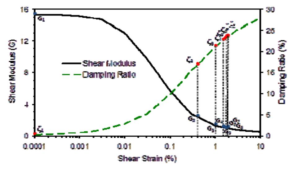
Figure 4. Strain-compatible shear modulus and damping iteration
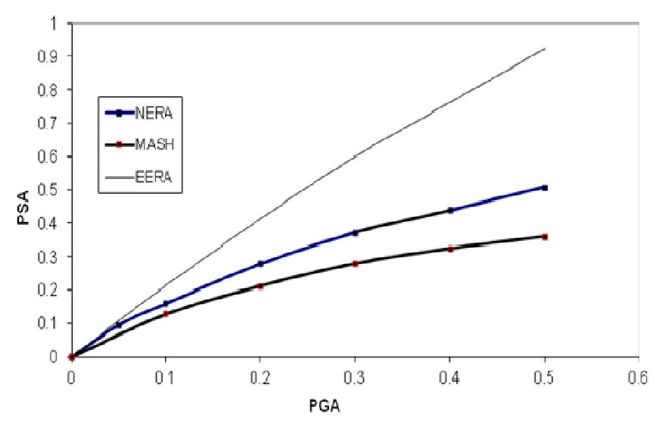
Figure 5. Linear and nonlinear models response
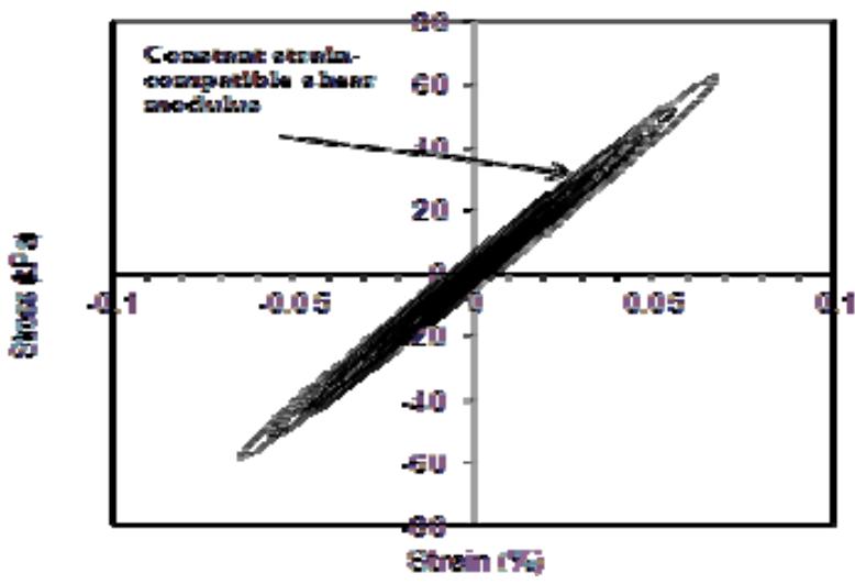
Figure 6. Linear stiffness responses in equivalent linear model
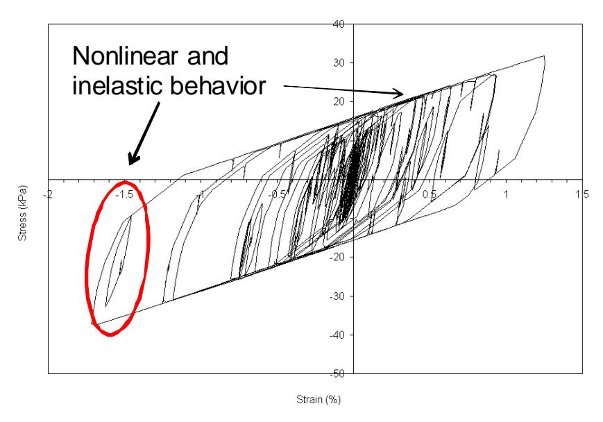
Figure 7. Nonlinear stiffness and inelastic response in nonlinear models
4.2 Proposed model features
Apriadi (2009a) and Apriadi et al. (2009b) have shown several model features of non-linear continuous hyperplasticity kinematic hardening MCC model in modeling cyclic behavior of soils such as irreversible unloadingreloading response, a hysteresis loop with accumulation shear strain and smooth transition of stiffness during unloading-reloading cycles as shown in Figures 7 and 8. It is clearly shown that the dominant hardening processes such that the Bauschinger effect can be represented very well. Moreover, the developed model can describe a non-linear behavior of soils more accurately across a wide range of strain amplitude.
However, over (normally) quite large numbers of cycles, the material also hardens isotropically such that the peak tension and compression stresses in a given cycle increase from one cycle to the next until saturation is achieved (Dunne and Petrinic, 2005). Such a process is represented schematically in Figure 9. Starting from the point of zero stress and strain, the material is subjected to the strain and then the stress increases until yield is achieved at point A, and the material kinematically hardens leading to the translation of the yield surface.
Dunne and Petrinic (2005) stated that once the peak strain is achieved, the strain reversal occurs so that the material becomes elastic at point B. Elastic deformation continues until the load point reaches the yield surface again at point C where plasticity recommences until the next strain reversal at point D. The yield surface is translated again because of the kinematic hardening. The stress–strain loop BCDB produced in this way is called a hysteresis loop. If, in addition to the kinematic hardening, the material also isotropically hardens, then superimposed upon the translation of the yield surface is a progressive expansion, shown by the broken line hysteresis loop in Figure 7. This process, by which the peak stress and strain in a hysteresis loop increase, due to isotropic hardening, is often called cyclic hardening, as it often occurs from cycle to cycle over many cycles. Kinematic hardening, on the other hand, occurs within each cycle.
This fact supports the importance of development of the mixed hardening MCC model in accordance to improve current constitutive models for evaluating the effects of local soil conditions on earthquake ground response analysis.
4. Conclusions
Based on the our current work on development of hyperplasticity-based model for predicting earthquake ground response analysis, some important conclusions can be drawn, i.e.:
- 1. Formulation of a non-linear mixed hardening multisurface hyperplasticity model considering a stiffness factors of the kinematic hardening of the yield surfaces proportional to the pre-consolidation pressure have been presented.
- 2. Some definitions of pre-consolidation pressure and recent constitutive modeling in ground response analysis have been also explained.
- 3. Remarks are made on the features of the proposed model such as irreversible unloadingreloading response, a hysteresis loop with accumulation shear strain and smooth transition of stiffness during unloading-reloading cycles.
- 4. Results of numerical implementation, simulations and model verification employing the proposedmathematical model formulation will be reported in a future publication.
- 5. This study is expected to contribute for improvement of load-deformation prediction in earthquake ground response analysis
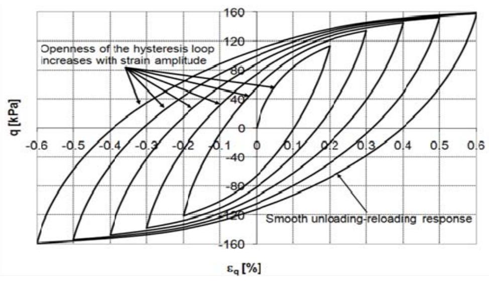
Figure 7. Cyclic undrained stress-strain curves (Apriadi et al., 2009)
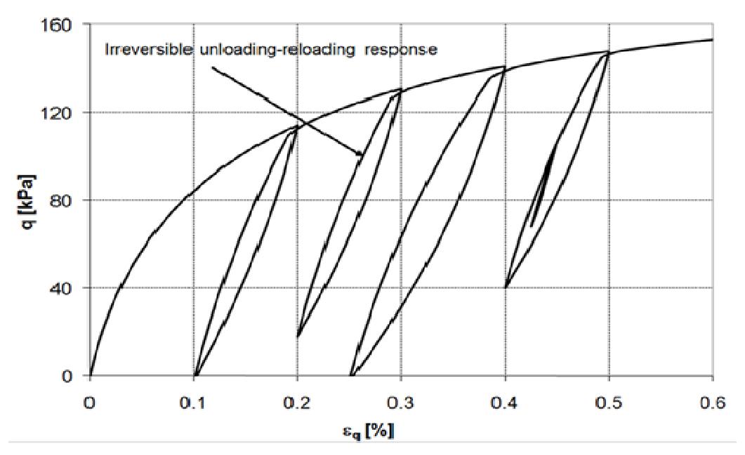
Figure 8. Irreversible cyclic undrained stress-strain curves (Apriadi et al., 2009)
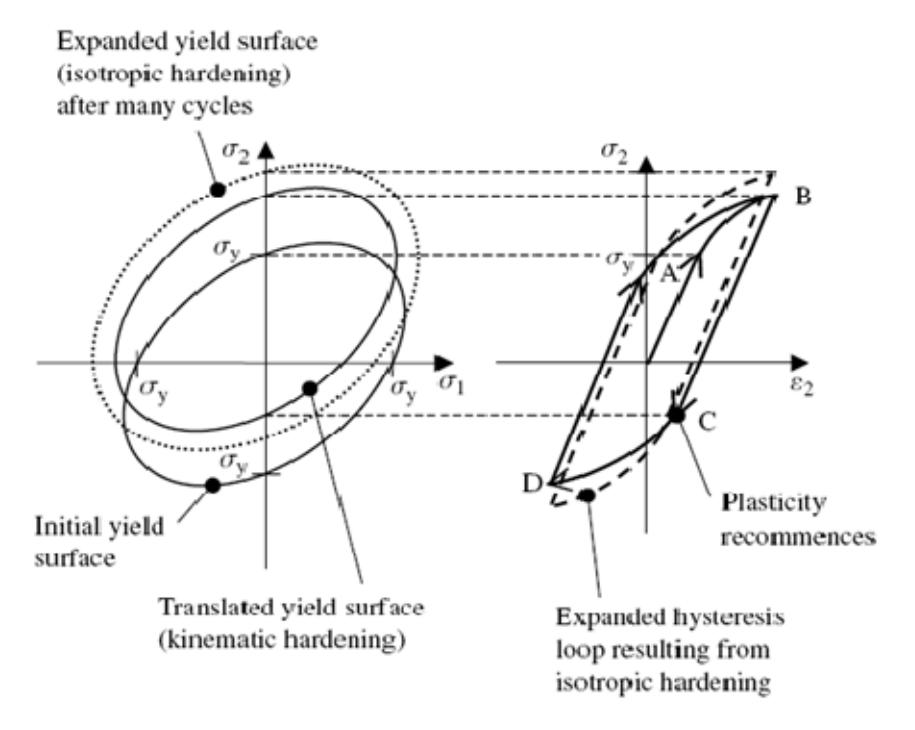
Figure 9. Mixed kinematic and isotropic hardening (Dunne and Petrinic, 2005)
5. Acknowledgements
This work was supported by AUN/SEED-Net JICA. The authors would like to express its sincere appreciation for the grant.