
1. Introduction
When the reservoir has been full for some time, conditions of steady seepage become established through the dam with the soil below the top flow line in the fully saturated state. This condition must be analysed in terms of effective stress with values of pore pressure being determined from the flow net. The factor of safety for this condition should be at least 1.5. Internal erosion is a particular danger when the reservoir is full because it can arise and develop within a relatively short time, seriously impairing the safety of the dam, (Edil, 1982).
Most slope failures occur either during, or at the end of construction. Pore water pressures depend on the placement water content of the fill and on the rate of construction. A commitment to achieve rapid completion will result in high pore water pressures at the end of construction. However, the construction period of an embankment dam is likely to be long enough to allow partial dissipation of excess pore water pressure, especially for a dam with internal drainage. Dissipation of excess pore water pressures can be accelerated by installing horizontal drainage layers within the dam. However, a total stress analysis would result in an over conservative design. An effective stress analysis is therefore preferred.
2. Methods
This Research is focused of the analysis slope stability on Dam Waduk Keuliling Kabupaten Aceh besar. The purpose about the topic consist of:
- a. The geometric of Dam and soil parameters such as indices soil properties, shear strength and soil permeability.
- b. The computation of finite Element Procedure are performd by utilizing of professional software Plaxis 7.1.1.
2.1 Finite element concept
The stage construction analysis of dam embankment in plane strain. Plaxis software were performed at triangular element with 15 nodal.
The general polynomial form of two components of displacement model is
\[u(x,y) = a_0 + a_1x + a_2y + a_3x^2 + a_4xy + a_5y^2 + a_6x^3 + a_7x^2y + a_8xy^2 + a_9y^3 + a_{10}x^4 + a_{11}x^3y + a_{12}x^2y^2 + a_{13}xy^3 + a_{14}y^4\] \[v(x,y) = b_0 + b_1x + b_2y + b_3x^2 + b_4xy + b_5y^2 + b_6x^3 + b_7x^2y + b_8xy^2 + b_9y^3 + b_{10}x^4 + b_{11}x^3y + b_{12}x^2y^2 + b_{13}xy^3 + b_{14}y^4\] (1)
Where u and v denote the components of displacement in the x and y directions.
2.1.1 Strain
The strain displacement equations for either plane stress or plane strain are given by Equation (2).
\[\varepsilon_{xx} = \frac{\partial u}{\partial x} = a_1 + 2a_3x + a_4y + 3a_6x^2 + 2a_7xy + 2a_8y^2 +\]popular in the linear elastic constitutive la Young's modulus and Poison's ratio, (Siriwardane, 1984). \[\varepsilon_{yy} = \frac{\partial u}{\partial y} = b_2 + b_4x + 2b_5y + b_7x^2 + b_8y^2 + 3b_9y^2 +\]\[b_{11}x^3 + 2b_{12}xy^2 + 3b_{13}xy^2 + 4b_{14}y^3\]\[\varepsilon_{yy} = \frac{\partial u}{\partial y} = b_2 + b_4x + 2b_5y + b_7x^2 + b_8y^2 + 3b_9y^2 +\]\[\varepsilon_{yy} = \frac{\partial u}{\partial y} = b_2 + b_4x + 2b_5y + b_7x^2 + b_8y^2 + 3b_9y^2 +\]\[\varepsilon_{yy} = \frac{\partial u}{\partial y} = b_2 + b_4x + 2b_5y + b_7x^2 + b_8y^2 + 3b_9y^2 +\]\[\varepsilon_{yy} = \frac{\partial u}{\partial y} = b_2 + b_4x + 2b_5y + b_7x^2 + b_8y^2 + 3b_9y^2 +\]\[\varepsilon_{yy} = \frac{\partial u}{\partial y} = b_2 + b_4x + 2b_5y + b_7x^2 + b_8y^2 + 3b_9y^2 +\]\[\varepsilon_{yy} = \frac{\partial u}{\partial y} = b_2 + b_4x + 2b_5y + b_7x^2 + b_8y^2 + 3b_9y^2 +\]\[\varepsilon_{yy} = \frac{\partial u}{\partial y} = b_2 + b_4x + 2b_5y + b_7x^2 + b_8y^2 + 3b_9y^2 +\]\[\varepsilon_{yy} = \frac{\partial u}{\partial y} = b_2 + b_4x + 2b_5y + b_7x^2 + b_8y^2 + 3b_9y^2 +\]\[\varepsilon_{yy} = \frac{\partial u}{\partial y} = b_2 + b_4x + 2b_5y + b_7x^2 + b_8y^2 + 3b_9y^2 +\]\[\varepsilon_{yy} = \frac{\partial u}{\partial y} = b_2 + b_4x + 2b_5y + b_7x^2 + b_8y^2 + 3b_9y^2 +\]\[\varepsilon_{yy} = \frac{\partial u}{\partial y} = b_2 + b_4x + 2b_5y + b_7x^2 + b_8y^2 + 3b_9y^2 +\]\[\varepsilon_{yy} = \frac{\partial u}{\partial y} = b_2 + b_4x + 2b_5y + b_7x^2 + b_8y^2 + 3b_9y^3 +\]\[\varepsilon_{yy} = \frac{\partial u}{\partial y} = b_2 + b_4x + 2b_5y + b_7x^2 + b_8y^2 + 3b_9y^3 +\]\[\varepsilon_{yy} = \frac{\partial u}{\partial y} = b_2 + b_4x + 2b_5y + b_7x^2 + b_8y^2 + 3b_9y^3 +\]\[\varepsilon_{yy} = \frac{\partial u}{\partial y} = \frac{\partial u}{\partial y} = b_2 + b_4x + 2b_5y + b_7x^2 + b_8y^3 + b_9y^3 +\]\[\varepsilon_{yy} = \frac{\partial u}{\partial y} = \frac{\partial u}{\partial y} = \frac{\partial u}{\partial y} = \frac{\partial u}{\partial y} = \frac{\partial u}{\partial y} = \frac{\partial u}{\partial y} = \frac{\partial u}{\partial y} = \frac{\partial u}{\partial y} = \frac{\partial u}{\partial y} = \frac{\partial u}{\partial y} = \frac{\partial u}{\partial y} = \frac{\partial u}{\partial y} = \frac{\partial u}{\partial y} = \frac{\partial u}{\partial y} = \frac{\partial u}{\partial y} = \frac{\partial u}{\partial y} = \frac{\partial u}{\partial y} = \frac{\partial u}{\partial y} = \frac{\partial u}{\partial y} = \frac{\partial u}{\partial y} = \frac{\partial u}{\partial y} = \frac{\partial u}{\partial y} = \frac{\partial u}{\partial y} = \frac{\partial u}{\partial y} = \frac{\partial u}{\partial y} = \frac{\partial u}{\partial y} = \frac{\partial u}{\partial y} = \frac{\partial u}{\partial y} = \frac{\partial u}{\partial y} = \frac{\partial u}{\partial y} = \frac{\partial u}{\partial y} = \frac{\partial u}{\partial y} = \frac{\partial u}{\partial y} = \frac{\partial u}{\partial y} = \frac{\partial u}{\partial y} = \frac{\partial u}{\partial y} = \frac{\partial u}{\partial y} = \frac{\partial u}{\partial y} = \frac{\partial u}{\partial y} = \frac{\partial u}{\partial y} = \frac{\partial u}{\partial y} = \frac{\partial u}{\partial y} = \frac{\partial u}{\partial y} = \frac{\partial u}\]
\[\gamma_{xy} = \frac{\partial u}{\partial y} + \frac{\partial v}{\partial x}\]
The strain displacement relations from Equations (2) of 15 node element U<sup>e</sup> is
\[\varepsilon = B U^e\] where : \(\varepsilon\) = strain vector.
The vector displacement of 15 node element U<sup>e</sup> as
\[\mathcal{E} = \begin{pmatrix} \mathcal{E}_{xx} \\ \mathcal{E}_{yy} \\ \gamma_{xy} \end{pmatrix} \text{ and } U^e = \begin{pmatrix} u_1 \\ v_1 \\ u_2 \\ v_2 \\ \vdots \\ \vdots \\ u_{15} \\ v_{15} \end{pmatrix}\] \[(3)\]
2.1.2 Compatibility equation
The relationship displacement \(\upsilon\), \(\nu\), axial strain \(\varepsilon_x\), \(\varepsilon_y\), engineering strain \(\gamma_{xy}\), in matrix form is:
\[\begin{bmatrix} -\frac{\partial}{\partial x} & 0\\ 0 & -\frac{\partial}{\partial y}\\ \frac{\partial}{\partial y} & \frac{\partial}{\partial x} \end{bmatrix} u = \begin{cases} \varepsilon_{x}\\ \varepsilon_{y}\\ \gamma_{xy} \end{cases}\] \[(4)\]
2.1.3 Constitutive law
Constitutive law determine the relationship between stress and strain is a continuum material properties mecanics, which is expressed by
\[\sigma = C\varepsilon \tag{5}\]
Above equation is the basis of the stress-strain relationship in the linear elastic constitutive law. The most popular in the linear elastic constitutive law is to use Young's modulus and Poison's ratio, (Desai and Siriwardane, 1984).
\[C = \frac{E}{\left(1+v\right)\left(1-2v\right)} \begin{bmatrix} (1-v) & v & 0 \\ v & (1-v) & 0 \\ 0 & 0 & \left(\frac{1-2v}{2}\right) \end{bmatrix}\] (6)
2.1.4 Boundary condition
Boundary condition can be provided for displacement (U) and stress (\(\sigma\)), as expression
\[\underline{U} = \left\{ \frac{\overline{u}}{v} \right\} \qquad \underline{\sigma} = \left\{ \frac{\overline{\sigma}_x}{\overline{\sigma}_y} \right\} \tag{7}\]
The relationship between total stress, effective stress and pore water pressure is
\[\begin{cases} \sigma_{xx} \\ \sigma_{yy} \\ \tau_{xy} \end{cases} = \begin{cases} \sigma'_{xx} \\ \sigma'_{yy} \\ \tau'_{xy} \end{cases} + \begin{cases}\nu \end{cases}\] (8)
\[\underline{\sigma} = \underline{\sigma}' + \underline{u} \tag{9}\]
\[\underline{\sigma}' = C\varepsilon + u \tag{10}\]
2.1.5 Element stiffnes matrix
Body force and surface traction that occurs on the elements inserted into the at the nodal point force. For a triangular element nodal force vector is
\[P^{e} = \begin{pmatrix} P_{1x} \\ P_{2y} \\ \dots \\ \dots \\ P_{15x} \\ P_{15y} \end{pmatrix}\] (11)
Where the nodal force will occur forces in the x and y direction, so that the relationship of nodal displacement in the matrix are
\[K^e U^e = P^e (12)\]
In form matrix element stiffness is:
\[K^e = \int B^T D.B.dv \tag{13}\]
2.1 Basic concepts applied to slope stability
The discovery of the principle of effective stress by Terzaghi in 1920s marks the beginning of modern soil mechanics. This concept is very relevant to problems associated with slope stability. Consider three principal stresses, \(\sigma_1\), \(\sigma_2\), and \(\sigma_3\) at any point in saturated soil mass and let u be the pore water pressure at that point. Changes in the total principal stresses caused by a change in the pore water pressure u (also called the neutral stress) have practically no influence on the volume change or on the stress condition for failure. Compression, distortion, and a change of shearing resistence result exclusively from changes in the effective stress, \(\sigma_1\), \(\sigma_2\), and \(\sigma_3\) which are defined as
\[s_1' = s_1 - u\] \(s_2' = s_2 - u\) \(s_3' = s_3 - u\) (14)
Therefore, changes in u lead to changes in effective stresses.
Slope Materials have a tendency to slide due to shearing stress created in the soil by gravitational and other force (e.g. water flow, tectonic stress, seismic activity). This tendency is resisted by the shear strength of slope material expressed by Mohr-Coulomb theory as shown in (Figure 1).
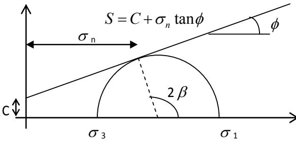
Figure 1. Shear Strength envelope (Abramson, et al, 1996)
\[\tau = c + \sigma_n \tan \phi \tag{15}\]
Where
\(\tau\) = total shear strength of soil
c = total cohession of soil
\(\sigma_n\) = total normal stress
\(\phi\) = total angle of internal friction
In term of effective stress;
\[\tau' = C' + (\sigma_n - u) \tan \phi'\] (16)
Where
\(\tau'\) = drained shear strength of the soil
C' = effective cohession
\(\sigma_N\) = normal stress
u = pore water pressure
\(\phi'\) = angle of internal friction in term of effective stress
2.2 Factor of safety concepts
The definition of Safety of Factor often considered is the ratio of total resisting forces to total disturbing (or driving) force for planar failure surfaces or the surface.
\[SF = \frac{\text{shear strength}}{\text{shear stress}}\] (17)
Where:
If, SF > 1.0 The slope will be stable
If,SF = 1.0 The slope will be tendency to unstable
If,SF < 1.0 The slope will be unstable
The carry out shear strength parameter is investigation and laboratorium soil test, therefore shear stress applied working load at the slope surface. Various definition Safety of Factor shown on Figure 2.
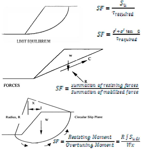
Figure 2. Various definitions of factor of safety (Abramson, et al, 1996)
The minimum factors of safety for embankment dams would be:
- 1. Upstream slope, range of safety factor after the end of construction condition is 1.3 1.5 and following rapid drawdown (slip circles between high and low water levels) 1.2 1.3 of SF.
- 2. Downstream Slope, Earthquake and reservoir full 1.2 of SF and reservoir full steady seepage condition 1.5 of SF.
- 3. The steady state condition in reservoir full
2.3 The ordinary method of slices
In this method, it assumed that the forces acting upon the sides of any slice have zero resultant in the direction normal to the failure are for that slice. This situation is show on Figure 3 below.
With this assumption,
\[\overline{N}_i = W_i \cdot \cos \theta_i - U_i = W_i \cos \theta_i - u_i \Delta l_i\] (18)
\[SF = \frac{c.L + \tan \phi \sum_{n=1}^{i=n} (W_i \cos \theta_i - u_i \Delta l_i)}{\sum_{n=1}^{i=n} W_i \sin \theta_i}\](19)
The back analysis with Ordinary Method of slices for sta 0+500 as follow; (Figure 4)
Table 1. Technical criteria for adequacy of design slope stability (Edil, 1982)
| No | Description | SF |
|---|---|---|
| 1 | Construction | 1.5 |
| 2 | Reservoir full | 1.5 |
| 3 | Sudden drawdown | 1.1 to 1.25 |
Figure 3. Forcer considered in ordinary method of slices (Edil, 1982)
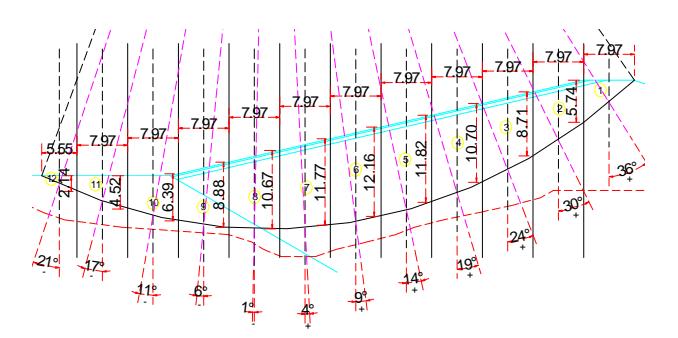
Figure 4. Slices at sta 0+500 dam keuliling
2.4 The analysis slope with Bishop's simplified method (1955)
In this metod, it is assumed that the forces acting on the sides of any slice have zero resultant in the vertical direction.
Sum force in vertical direction and the variation of x across a slice is ignore. i.e. \(X_n - X_{n+1} = 0\).
\[Fv = 0 = -N_n \cos \alpha_n - (Sm)n \sin \alpha_{n+} W_{n+}(X_{n-}X_{n+1}) = 0\] (20)
Assume, \(X_n - X_{n+1} = 0\); Subtitute \(S_n/F\) for \((S_m)n\); solve for \(N_n\)
Subtituting Nn in the original equation for F, We obtain
\[SF = \frac{\sum \{ [c_n, b_n + (w_n - u_n, b_n) \tan \phi c_n - (1/m_\alpha) \}}{\sum w_n \sin \alpha c_n}\](21)
Where
\[m_{\alpha} = \cos \alpha [1 + (\tan \alpha_n \tan \alpha_n^f)/F] = \cos \alpha_n + \frac{\sin \alpha_n \tan \alpha_n^f}{F}\] (22)
Since F appears on both sides of the equation 6, it is most convenient to solve for F in an iterative manner. It is useful to have \(m_{\alpha}\) plotted for any assumed value of SF, as shown in Figure 5.
2.5 The Analysis slope with finite element methods
The finite element method is a method for numerical solution of field problem. A field problem requires that to determine the spatial distribution of one or more dependent variable. Then, to find the distribution of force in soil material, or the distribution of displacements and stresses in the slope. Mathematically, a field problem is described by differential equations or by an integral expression. Either description may be used to formulate finite elements. Finite element formulations, in software are contained in general purpose finite element analysis program (e.g PLAXIS).
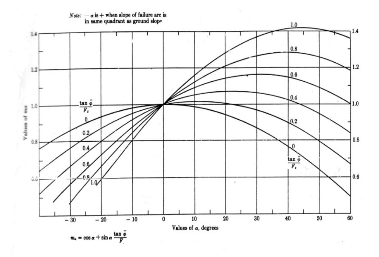
Figure 5. Values of m<sub>α</sub> for use in calculation (Edil, 1982)
PLAXIS is a finite element package specifically intended for the analysis of deformation and stability in geotechnical application require advanced constitutive models for the simulation of the non-linier and time-dependent behaviour of soils. in addition, since soil is multi-phase material, special procedures are required to deal with hydrostatic and non hydrostatic pore pressure in the soil. Although the modeling of the soil itself is an important issue, many geotechnical engineering projects involve the modeling of structures and the interaction between the structure and the soil
2.6 The safety analysis
In design of an embankment, it is important to consider not only the final stability, but also the stability during construction. The Strength parameter \(c'_f\) and \(\phi'_f\) is
\[c'_f = \frac{c'}{SF} \tag{23}\]
\[\phi'_{f} = \arctan\left(\frac{\tan\phi'}{SF}\right) \tag{24}\]
The safety of factor is traditionally defined as a ratio of actual soil shear strength to the minimum shear
strength required to prevent failure [Bishop, 1955]. SF is the factor by which the soil shear strength must be divided to bring the slope to the verge of failure. The resulting factor of safety is the ratio of the soil's actual shear strength to the reduced shear shear strength at failure (Abramso, et al., 1996).
2.7 Method analysis safety factor (ΣMsf) in Plaxis
A safety analysis in PLAXIS can be executed by reducing the strength parameters of the soil. This process is called Phi-c reduction. If safety analysis performed by means of Phi-c reduction on a geometry where advanced soil models are used, then these models are transformed into Mohr-Coulomb using a constant stiffness modulus based on the actual stress level at the beginning of the analysis. This option is a separate loading type which can be selected from the Loading input inbox in a Plastic calculation using the manual control or number of steps procedure.
Phi-c reduction is an option that is available in PLAX-IS to compute safety factor. This option is only available for plastic calculation using the manual control or the load advancement number of steps procedure. In the Phi-c reduction approach the strength parameters tan f and c of the soil are successively reduced until failure of the structure occurs. The strength of structural objects like beams and ancors is not influenced by Phi-c reduction.
The Total multiplier \(\Sigma\)Msf is used tu define the value of the soil strength parameters at a given stage in analysis:
\[\sum Msf = \frac{\tan \phi_{input}}{\tan \phi_{reduced}} = \frac{c_{input}}{c_{reduced}}\](25)
Where the strength parameters with the subscript 'input' refer to the properties entered in the material sets and parameters with the subscript 'reduced' values used in the analysis. In contrast to other total multipliers, \(\Sigma Msf\) is set to 1.0 at the starts of calculation to set all material strength to their un reduced values. The strength parameters are successively reduced automatically until failure of the structure occurs. At this point the factor of safety is given by:
\[Safety \text{ factor} = \frac{S_{\text{maximum available}}}{S_{\text{needed for equilibrium}}}\] (26)
Where S represents the Shear strength. The ratio of true strength to the compute minimum strength required for equilibrium is the safety factor that is conventionally used in soil mechanic. By introducing the standard Coulomb condition, the Safety factor is obtained:
\[Safety \text{ factor} = \frac{c + \sigma_n \tan \phi}{c_r + \sigma_n \tan \phi_r}\] (27)
Where c and \(\phi\) are input strength parameters and \(\sigma_n\) is the actual normal stress component. The parameters \(c_r\) and \(\phi\) r are reduced strength parameters that are just large enough to maintain equilibrium.
When using Phi-c reduction in combination with advanced soil model, these models with actually behave as a standard Mohr-Coulomb model, since stress dependent stiffness behaviour and hardening effects are excluded from the analysis.
2.8 The simulation of embankment construction in PLAXIS
The Embankment is simulated with Plaxis in plane strain, using small-strain mode (the coordinates of the nodes are updated according to the compute nodal displacement). The soil is modeling as a linier elastic perfectly plastic material with a Mohr coulomb yield condition and an associated flow rule. The Stage construction Modelling in Plaxis as:
Step-1: In order to perform finite element analysis, the geometry of Dam embankment has to be defined into mesh element.
Step-2: To defined Model parameter Input in PLAXIS
Step-3: Initial condition
Step-4: Stage construction of Embankment
Step-5: The Analysis end of Construction of Embankment
Step-6: The Minimun Potential pore pressure analysis for long term Condition.
Step-7: The Safety Factor Analysis for Long term
Step-8: The full reservoir at elevation 9.8 metre of sta 0+500 to sta 0+600.
Step-9: The Rapid Drawdown Analysis When the reservoir full
Step-10: The Analisis Safety Factor for under rapid drawdown condition.
All the embankment alnalysis as follow: (Table 1)
2.9 Soil Modelling
The Mohr-Coulomb yield condition of Coulomb's friction law to general states of stress. In fact, this condition ensures that Coulomb's friction law is obeyed in any plane within a material element. The full Mohr-Coulomb yield condition can be defined by three yield functions when formulated in terms of principal stresses. Two plastic model parameters appearing in the yield functions are the well known friction angle \(\phi\) and c. These yield functions together represent a hexagonal cone in principal stress space as shown in Figure 3.
In addition to the yield functions, three plastic potential functions are defined for the Mohr-Coulombs:
\[\tau - \sigma \tan \phi - c = 0\];
\[\frac{\sigma_{1-} \sigma_3}{2} = \frac{\sigma_1 + \sigma_3}{2} \sin \phi + c.\cos \phi \tag{28}\]
Table 1. The simulation of stage construction embankment at sta 0 +500 to sta 0 + 600
| No | Stage Construction | Hight of Embankment (m) | Ground Water Table (m) |
|---|---|---|---|
| 1 | Embankment level 1 | 4 | 2 |
| 2 | Embankment level 2 | 5 | |
| 3 | Embankment level 3 | 4 | |
| 4 | Embankment level 4 | 4 | |
| 5 | Embankment level 5 | 2 | |
| 6 | Embankment level 6 | 2 | |
| 7 | Embankment level 7 | 3 | |
| 8 | Embankment level 8 | 1 |
Figure 6. The Mohr-Coulomb vield surface in principal space (c=0) (Brinkgreve, et al. 1998)
The hardening-soil model is an advanced model for simulating the behaviour of different type of soil, both soft soil and stiff soil. When subjected deviatoric loading, soil shows as decreasing stiffness and simultaneously irreversible plastic strains develop. In the special case of a drained triaxial test, the observed relationship between the axial strain and the deviatoric stress can be well approximated by a hyperbola.
A basic idea for the formulation of the hardening-soil is the hyperbolic relationship between the vertical strain, \(\varepsilon_1\), and the deviatoric stress, q, in primary triaxial loading. Here standard drained triaxial tests tend to yield curves that can be described by:
\[-\varepsilon_{1} = \frac{1}{2E_{50}} \frac{q}{1 - q/q_{a}} \text{ untuk } q < q_{f}\] (29)
Where \(q_a\) is the asymptotic value of the shear strength. This relationship is plotted in Figure 4. The parameter E<sub>50</sub> is the confining stress parameter dependent stiffness modulus for primary loading.
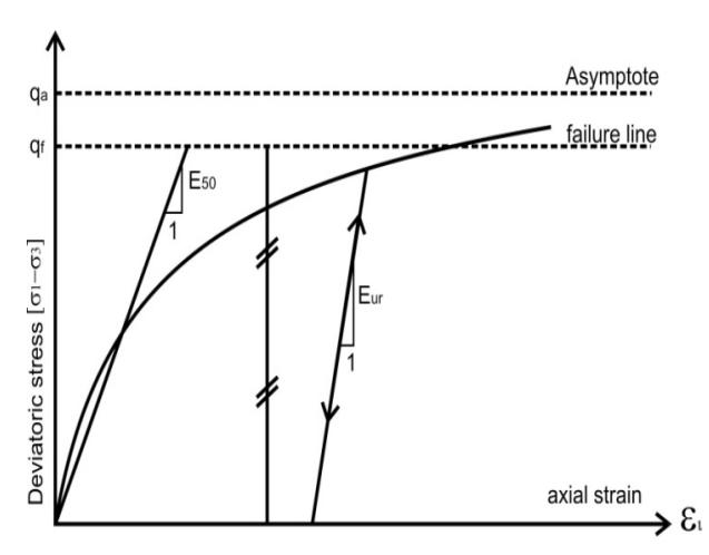
Figure 7. Hyperbolic stress-strain relation in primary loading for a standard drained triaxial test (Brinkgreve, et al. 1998)
3. Geotechnical Condition and Selected Parameters
3.1 The present condition of soil parameters
The layer structure consists of mixture soil, silt, sandy clay 1 - 2.5 m at depts between 1 to 2.5 m. Below this layer there is a weathered rock layer with a thickness of 5 to 12 meters. Permeability zone is the order of 10<sup>-1</sup> <sup>4</sup> cm / sec. Below this zone there is a fairly hard rock with a thickness ranging from 27.5 metre with a permeability order of 10<sup>-4</sup> cm / sec. Rock consists of sandstone with a thin insertion of 20 cm stone clay, silt stone
3.2 Geometry of dam
Geometry Reservoir Dam Keuliling Aceh Besar district and zone arrangement material is as shown below: (Figure 8).
Filter is used to control the seepage should have pore sizes small enough to prevent particle-borne and permeability must be high enough so that the flow can bypass the filter quickly.
3.3 Input parameters in the analysis
In Plaxis software, soil properties and material properties of structures are stored in material data set. A data set for soil generally represents a certain soil layer and can be assigned to the corresponding cluster in the geometry model. The data set each soil layer as follow:
3.4 The analysis with ordinary method of slices
The Figure of slice at sta 0+500 shown in Figure 4 as follow: (Table 9)
Table 7. Parameters of Mohr Coulomb model (Wahana Adya Konsultan, 2000)
| Zone 3 | Zone 3 +4 | Zone 8 | |||
|---|---|---|---|---|---|
| Type | Drained | Drained | Drained | ||
| \(\gamma_{dry}\) | \[kN/m^3\] | 17.52 | 21 | 20 | |
| \(\gamma_{dry}\) | \[kN/m^3\] | 20.60 | 22 | 21 | |
| \(k_x\) | m/day | 12 | 15 | 100 | |
| \(k_y\) | m/day | 12 | 15 | 100 | |
| υ | 0.15 | 0.15 | 0.22 | ||
| C | kPa | 30 | 30 | 31518 | |
| \[\varphi_{ref}\] | Degree | 30.3 | 30.3 | 42 | |
| E50 | kPa | 20,000.00 | 20,000.00 | 1,260,720.00 | |
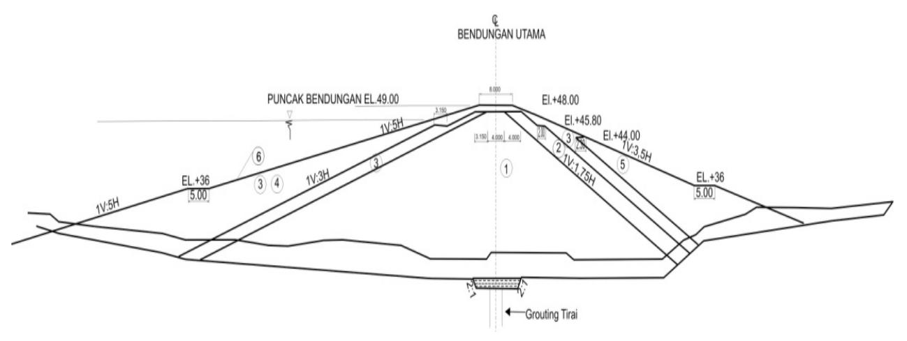
Figure 8. Geometry Dam of Waduk Keuliling (Wiratman & Associates, 2002)
Table 8. The soil parameters of Hardening model
| Parameters | Unit | Layer 1 | Layer 2 | Zone 1 | Zone 2 | Zone 5 |
|---|---|---|---|---|---|---|
| type | undrained | undrained | undrained | drained | Drained | |
| \(\gamma_{\rm dry}\) | kN/m3 | 17.4 | 17.7 | 15.5 | 17 | 18.95 |
| \(\gamma_{\rm dry}\) | \(kN/m^3\) | 20.8 | 20.59 | 19.1 | 20 | 18.95 |
| \(k_x\) | m/day | 0.312 | 0.506 | 0.0153 | 8 | 14 |
| \(k_{v}\) | m/day | 0.312 | 0.506 | 0.0153 | 8 | 14 |
| Ý | 0.2 | 0.2 | 0.2 | 0.2 | 0.2 | |
| C | kPa | 48 | 40 | 45 | 1 | 2 |
| Φ | Degree | 42.9 | 43 | 29.4 | 34 | 35 |
| \({\rm E_{50}}^{\rm ref}\) | kPa | 73,114.07 | 32,258.00 | 34,000.00 | 38,500.00 | 52,000.00 |
| \(E_{oed}^{ref}\) | kPa | 73,114.07 | 31,591.77 | 12,491.63 | 35,000.00 | 52,000.00 |
Table 9. Back Analysis of Ordinary Method of Slice
| Slice | Δχί | Average | θi (degrees) | W₁.sin O₁ | Wi.cos Θi | L |
|---|---|---|---|---|---|---|
| (m) | height (m) | (kN/m) | (kN/m) | (m) | ||
| 1 | 7.97 | 5.74 | 36 | 471.1 | 648.4 | 9.85 |
| 2 | 7.97 | 7.23 | 30 | 504.4 | 873.7 | 9.20 |
| 3 | 7.97 | 9.71 | 24 | 551.2 | 1,238.0 | 8.72 |
| 4 | 7.97 | 11.26 | 19 | 511.9 | 1,486.6 | 8.43 |
| 5 | 7.97 | 11.99 | 14 | 405.0 | 1,624.5 | 8.21 |
| 6 | 7.97 | 11.97 | 9 | 261.4 | 1,650.2 | 8.07 |
| 7 | 7.97 | 11.22 | 4 | 109.3 | 1,562.9 | 7.99 |
| 8 | 7.97 | 9.78 | 1 | 23.8 | 1,364.7 | 7.97 |
| 9 | 7.97 | 7.64 | -6 | -111.4 | 1,060.3 | 8.01 |
| 10 | 7.97 | 5.46 | -11 | -145.3 | 747.7 | 8.12 |
| 11 | 7.97 | 3.33 | -17 | -135.9 | 444.7 | 8.33 |
| 12 | 5.55 | 1.07 | -21 | -37.3 | 97.1 | 5.94 |
| ] | Γotal | 2,408.10 | 98.86 |
\[SF = \frac{30*98.86}{2,408.10} = 1.23\]
The safety factor with the ordinary method of slice was obtain 1.23.
3.5 The analysis with Simplified Bishop method of slices
The method was first described by Bishop (1955). The analysis this method use Equation (21) and requires a trial and error solution. Since SF appears on both sides of the equation. The chart on Figure 3 can be used evaluated the function \(m_{\alpha}\).
3.6 The analysis with Plaxis
The Simulation phase of dam construction will be done by gradual accumulation. Behavior all conditions in the field of construction is an absolute that must be represented into conditions in the analysis.
| Clies W | 1A/ 1A/:: A: / | (2) ton A | (2).(4) | \(\mathbf{m}_a\) | (5)/(6) | |||
|---|---|---|---|---|---|---|---|---|
| Slice | Slice Wi | Wi-ui.∆xi | (3).tan ф | (2)+(4) | SF=4.3 | SF=4.35 | SF=4.3 | SF= 4.35 |
| (1) | (2) | (3) | (4) | (5) | (6) | (7) | ||
| 1 | 801.5 | 801.5 | 468.36 | 707.46 | 1.080 | 1.079 | 655.1 | 655.7 |
| 2 | 1,008.86 | 1,008.9 | 589.53 | 828.63 | 1.068 | 1.067 | 775.9 | 776.5 |
| 3 | 1,355.15 | 1,355.2 | 791.89 | 1,030.99 | 1.055 | 1.055 | 977.0 | 977.6 |
| 4 | 1,572.28 | 1,572.3 | 918.77 | 1,157.87 | 1.044 | 1.044 | 1,108.8 | 1,109.4 |
| 5 | 1,674.22 | 1,674.2 | 978.33 | 1,217.43 | 1.033 | 1.032 | 1,178.7 | 1,179.1 |
| 6 | 1,670.73 | 1,670.7 | 976.29 | 1,215.39 | 1.021 | 1.021 | 1,190.1 | 1,190.4 |
| 7 | 1,566.70 | 1,566.7 | 915.50 | 1,154.60 | 1.009 | 1.009 | 1,143.8 | 1,143.9 |
| 8 | 1,364.93 | 1,364.9 | 797.60 | 1,036.70 | 1.002 | 1.002 | 1,034.2 | 1,034.3 |
| 9 | 1,066.11 | 1,066.1 | 622.98 | 862.08 | 0.986 | 0.986 | 874.5 | 874.4 |
| 10 | 761.71 | 761.7 | 445.10 | 684.20 | 0.974 | 0.974 | 702.4 | 702.2 |
| 11 | 464.98 | 465.0 | 271.71 | 510.81 | 0.960 | 0.961 | 531.9 | 531.7 |
| 12 | 104.04 | 104.0 | 60.80 | 227.30 | 0.951 | 0.952 | 238.9 | 238.8 |
| 10,411.42 | 10,413.79 | |||||||
Table 10. The back analysis for Simplified Bishop method of slice
For assumed SF = 4.3 ; SF = \[\frac{10,411.42}{2,408.10}\] = 4.32 and \[SF = \frac{10,413.79}{2,408.10}\] = 4.32
A trial with SF = 4.3 would give SF = 4.32.
The end of construction showed a condition of increased shear strength based on the value of effective stress and 693.59 kN/m<sup>2</sup> excess pore water pressure at 319.56 kN/m<sup>2</sup>. Shear strength that occurs when the construction has finished and save against slopes failure.
The Plaxis performed with 15-node and triangle element. The distribution of nodes over the element shown in Figure 9. During a finite element calculation, displacement are calculated at the nodes. Nodes may be preselected for the generation of load-displacement curve.
Displacement that occurred during the construction period at the end of element 228 (at crest dam) in dam cores obtained a total displacement of 0.5 cm, the vertical displacement of 0.5 cm and 0.12 cm in the horizontal direction, is of little value so that the construction of the dam is safe against avalanches. Total deposits decreased from phase 1 to complete construction is 49.3 cm. In this condition obtained safety factor of 2.532 at the upper weir and SF = 2.518downstream weir. This shows that the construction is stable because the SF> 1.5.
3.6.1 Steady state condition
In this condition after the end of the dam construction in undrained conditions by providing a reservoir of water load on the dam with a height of 9.8 meters of water level upstream weir and 3 meters level water downstream.
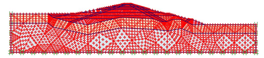
Figure 9. Plaxis Shown of number nodal and element
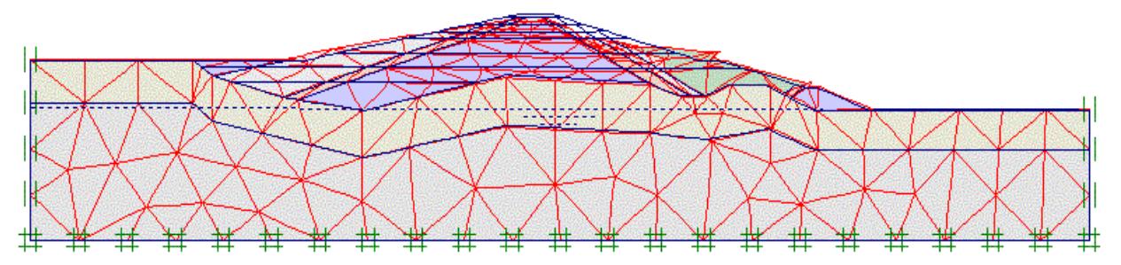
Figure 10. The mesh of element modeling of Dam sta 0+500
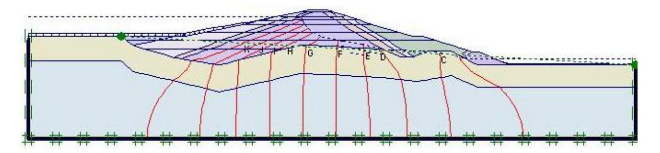
Figure 11. Steady state condition for flownet of output Plaxis
Seepage occurs when the dam reservoir in steady state conditions
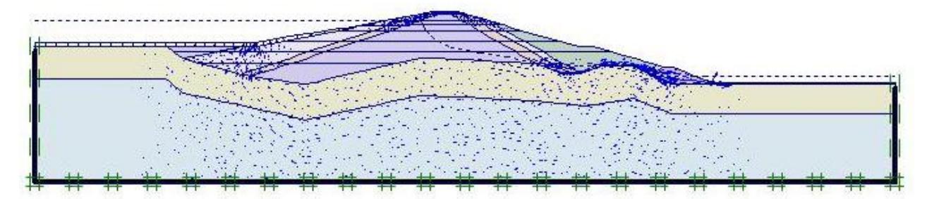
Figure 12. The Safety factor at seepage occurs in the steady state condition of output Plaxis
The amount of seepage at the dam body occurs at the speed \(4.16 \times 10^{-3} \text{ m}^3/\text{day/m}\) seepage maximum \(4.33 \times 10^{-3} \text{ m}\) / day. In this condition the stability of slopes upstream and downstream the weir is still stable with a safety factor of 2.514 is obtained on the slopes of upstream and downstream slopes of 2.516.
3.6.2 Longterm condition
In the long term this analysis by assuming the parameters are used effectively and the weir has been experiencing a consolidation. Displacement 32.6 cm in the vertical direction, horizontal direction of 0.6 cm and a total displacement of 32.70 cm. 748.44 kN/m<sup>2</sup> effective stress and excess pore pressure 8.88 kN/m<sup>2</sup>. Thus there is a decrease in dam body was 32.6 cm.
In this condition indicates that the shear strength increases and body so that the dam is stable with safety factor of 2.802 on the slopes of the dam upstream and 2.852 in the downstream weir.
3.6.3 Piping on the Dam
Harza (1984) The structure of the dam must be stable against piping. Safety factor for piping expression as:
\[SF = \frac{i_{critis}}{i_{exit}}\]
3.6.4 Control of piping
Data of laboratory tests on core material from a sample Bor dam OB-5 at a depth of 12 meters is
Gs = 2,667, e = 0,772.
\[\gamma_{sat} = \frac{(G_s + e)\gamma_w}{1 + e} = 19,407kN/m^2\]
\[i_{cr} = \frac{\gamma'}{\gamma_w} = 0,9407\]
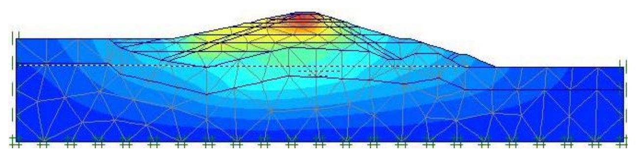
Figure 13. Longterm Analysis
\[i_{exit} = \frac{\Delta h}{L}\]
Where : \(\Delta h\) = head lost between two equipotential line. L = Leng of the low on one element. The elemen 179 at Sta 0 + 500 the seepage velocity = 4,38 E-3 m/ day, k = 0.0153 m/day.
\[i_{exit} = \frac{v}{k} = \frac{4,38x10^{-3}}{0,0153} = 0,286\]
\[SF = \frac{i_{critis}}{i_{crit}} = \frac{0.9407}{0.286} = 3,29\]
The SF on the condition that allowed piping is 3 to 4, then based on the results of the analysis above piping stable condition with a safety factor of 3.29.
4. Conclusion
- 1. Stability of the dam from the construction end of construction for sta 0+500 to sta 0+600 is 2.3 - 2.5. The long term condition safety factor is 2.78 -2.88. The rapid draw down condition show will stable, because the resulting safety factor is 2.2-2.4.
- 2. The Stability analysis with Ordinary method of slice is 1.23of SF and 4.32 the carry out safety factor with the bishop method.
- 3. In piping condition that occurs in unstable dam with a safety factor of 3.6 on average in the dam core. This value must match those required by the Safety factor between 3 and 4.
- 4. Dam is safe against the slopes failure in accordance with the requirements of specification of weir.