
Abstrak
Penelitian ini adalah tentang penentuan koefisien kekasaran Manning talang PVC (Polyvinyl Chloride), dan penentuan kapasitas talang akibat perubahan kemiringan memanjang saluran. Koefisien kekasaran dan kemiringan memanjang dasar saluran merupakan dua faktor yang sangat berpengaruh terhadap kecepatan dan kedalaman aliran suatu saluran. Oleh karena itu, dilakukanlah percobaan di laboratorium menggunakan sebuah talang PVC yang kemiringannya dapat diatur. Rumus yang digunakan adalah rumus Manning yang merupakan fungsi dari kecepatan aliran, koefisien kekasaran saluran, kedalaman aliran (geometri penampang basah saluran), dan kemiringan memanjang saluran. Air dipasok oleh sebuah pompa, dan debit alirannya ditentukan dengan menampung air yang keluar di ujung hilir saluran dengan sebuah ember. Volume air ember dan lama waktu yang diperlukan diukur. Kedalaman aliran diukur dengan mistar (ukuran lain geometri saluran adalah tetap, yaitu panjang 4m, lebar 12cm, tinggi 10cm). Pengukuran dilakukan lima kali untuk setiap perubahan kemiringan memanjang saluran dengan tahapan kemiringan 1cm/4m (dari 1cm/4m sampai 10cm/4m). Hasil percobaan menunjukkan nilainilai koefisien kekasaran Manning talang air PVC berkisar antara 0,010 sampai 0,014. Akibat peningkatan kemiringan dari 1cm/4m ke 10cm/4m, kedalaman aliran turun sampai 60% (tinggal 40%) untuk debit yang sama.
Kata-kata Kunci: Koefisien kekasaran, talang, PVC, Manning, kemiringan saluran.
1. Introduction
Chow (1973), Dingman (2009), Brater et al (1996), Mays (2001, 2011), and FSL (2013) reported lists of the values of the Manning roughness coefficient for channels made from various materials. However, the coefficients for some materials were not available in the lists. One of them is for open channels made from Polyvinyl Chloride (PVC). Based on the Manning formula, for other materials unspecified in the lists can be determined by undertaking an experiment in the laboratory. For example, Djajadi (2009) investigated some Manning roughness coefficients for a prismatic trapezoidal-shaped channel in the laboratory. A brick-made channel was then lined with four different surfaces, i.e. plaster only, and three aggregate-attached plasters, i.e. aggregates with small, medium, and large sizes. The results were about 0.013, 0.019, 0.021 and 0.028 respectively for Manning roughness coefficients. Djajadi contributed at least one n value, i.e. for a plasterlined channel, because the three others need to be specified in more detailed what kind of roughness they are. This is due to Djajadi was more concerned in composite roughness coefficients instead of the homogeneous ones. Additionally, previous studies regarding PVC-made channels were reported by Mays (2000, 2011), Sturm (2001) and Kay (2008), but these focused on pipes.
Probably, the channel roughness coefficients made from one of these materials of plastic, rubber, and glass are next to those made from PVC. Linsley and Franzini (1979) listed both plastic and rubber for 0.009, French (1986) listed glass for 0.009 to 0.013, Chanson (2004) listed both glass and plastic for 0.010. A special note is given to Gribbin (2007) who reported PVC for 0,007 to 0,011, but for closed culverts. As a result, the objectives of the present study are: (1) to develop a physical model using a PVC gutter with slope adjusters (see Figure 1); (2) to measure the variables of the Manning formula, i.e. the flow rate and flow depth to predict the values of the Manning roughness coefficient for PVC gutters. Mays (2001) listed some Manning roughness coefficients for gutters, but none of them was specifically for a PVC gutter.
The values of the Manning roughness coefficient for PVC gutters are important things and can be used to design a gutter effectively using PVCmade materials. The present experiment is undertaken in the Laboratory of Fluid Mechanics and
Hydraulics, Civil Engineering, the University of Andalas. The gutter used is made from PVC with brand of "Maspion", type AW (white color). The flow discharge used is supplied by a pump which is continuously working along the experiment.
2. Formulation
As can be seen in Figure 1, this model uses a standard PVC gutter with dimensions of length L=4 m, width b=12 cm, height h=10 cm. The gutter is supported by a metal-made frame, and the gutter slope along the flow direction is adjustable to a need. On the end of the gutter upstream, a stilling tank is installed. Both the gutter and tank are sealed using silicone glue. Meanwhile on the end of the gutter downstream, the water falls freely into the receiver tank. The water is pumped into the stilling tank.
To determine the flow rate Q, the water coming out at the end of the downstream is collected using a bucket. Both the volume of water in the bucket V and the time required to fulfill the bucket Dt are measured. This is done five times for every single position slope S, written
\[Q = \frac{1}{5} \sum_{i=1}^{5} \frac{V_i}{\Delta t_i}\] (1)
The height of water in the gutter y measured using a ruler. Measurements are taken when the situation is steady and the water levels are the same at some points in the middle of the gutter, so the hydraulic variables of the gutter like a wet area A and wet perimeter P of the cross-section can be determined by
\[A = by = 0.12y \tag{2}\]
\[P = b + 2y = 0.12 + 2y \tag{3}\]
Figure 1. Sketch of a PVC gutter with slope adjusters
The hydraulic radius R is then defined by the wet cross-section area A divided by the wet crosssection perimeter P, written
\[R = \frac{A}{P} \tag{4}\]
As referred by Dingman (2009), an Irish engineer Robert Manning in 1889 developed an empirical formula for the computation of uniform flow in an open channel which has now been modified into the well known form, that is
\[Q = \frac{1}{n} A R^{\frac{2}{3}} S^{\frac{1}{2}} \tag{5}\] where Q is the flow rate obtained in Equation (1) in \(m^3/s\), n is the Manning roughness coefficient, A is the wet cross-sectional area in m<sup>2</sup> obtained in Equation (2), R is the hydraulic radius in m as defined by Equation (4), and S is the longitudinal slope of the channel base in m/m.
All variables in Equation (5) are already known except the roughness coefficient n. As mentioned above, variables A, R dan S can be quantitatively measured. However, the n value has to be determined by undertaking a laboratory work as did by Djajadi (2009). Therefore, this equation will be convenient if written as
\[n = \frac{1}{O}AR^{\frac{2}{3}}S^{\frac{1}{2}} \tag{6}\]
If the flow is at the critical state, the velocity head is equal to half the hydraulic depth, written
\[\frac{v^2}{2g} = \frac{D}{2} \tag{7}\]
The hydraulic depth D is defined as the ratio of the wet cross-section area A to the top width. In the case of a rectangular channel, the value of the top width is equal to that of base width b, so that, the value of the hydraulic depth is equal to that of the flow depth. Substitute Equation (2) and D = y into Equation (7), and then simplify giving
\[y = \sqrt[3]{\frac{Q^2}{b^2 g}} = y_c \tag{8}\] where \(y_c\) is the water depth at the critical state of flow. If the flow depth predicted by Equation (8), that is \(y_c\), is bigger than the measured flow depth, that is y, the flow is then at the super-critical state, and otherwise is at the sub-critical state.
3. Collection of Data, Calculation, and Analysis
As mentioned before, every variation of the base slope of the gutter, the flow depth y, and both the volume of water in the bucket V and the time required Dt to determine the flow rate Q are measured five times. There are 10 variations of the slopes with a 1 cm / 400 cm step. All of them are done continuously, and the pump is also working continuously without any disturbing. The measurement results for the water depths in the gutter, the volume of water in the bucket, and the time required, and also the resulting flow rates are shown in Table 1
The next step is to predict the Manning roughness coefficient n using the flow depths y and the flow rates Q in Table 1, and using Equations (2), (3), (4), (6), (8), this results in as shown in Table 2.
Based on Tabel 2, the relationship between the gutter slopes S and the roughness coefficients nare shown in Figure 2 (bold line).
In Figure 2 can be seen that the values of the roughness coefficient are not fixed if the slopes are varied. The values of the roughness coefficient tend to increase when the slopes are mild. However, when the slopes over 5 cm / 400 cm (or 0,0125 cm/cm), the roughness coefficients tend to stable at the range of 0.010 to 0.011. In the view of the state of flow, the roughness coefficients are more stable at the super-critical state instead of at the sub-critical one.
The flow rates are measured five times in every slope stage. The gutter slopes are varied into 10 stages, so that there are 50 times of the flow rates measured. Due to all measurements are undertaken continuously, so that the average of all flow rates can be obtained by its arithmetic average, i.e.,
\[\overline{Q} = \frac{1}{50} \sum_{i=1}^{50} Q_i = 689,5 \text{ cm}^3/\text{s}.\]
If the last average flow rate is used, the relation of the roughness coefficients and the slopes can be plotted as shown in Figure 2 (thin line), and the computation process is shown in Table 3.
Table 1. The measurement results for the water depths y in the gutter, the volume of water V in the bucket, and the time required Dt to determine flow rates Q
| y (cm) | V (cm3 ) | ∆ t (s) | Q (cm3 /s) | i | y (cm) | V (cm3 ) | ∆ t (s) | Q | |||
|---|---|---|---|---|---|---|---|---|---|---|---|
| i | (cm3 /s) | ||||||||||
| measured | measured | measured | calculated | measured | measured | measured | calculated | ||||
| S measured in 1cm/400cm | S measured in 2cm/400cm | ||||||||||
| 1 | 2,40 | 1170 | 1,82 | 643 | 1 | 1,90 | 1100 | 1,72 | 640 | ||
| 2 | 2,40 | 1280 | 1,94 | 660 | 2 | 1,90 | 1260 | 1,81 | 696 | ||
| 3 | 2,40 | 1170 | 1,75 | 669 | 3 | 1,90 | 1310 | 2,00 | 655 | ||
| 4 | 2,40 | 1360 | 1,90 | 716 | 4 | 1,90 | 1150 | 1,72 | 669 | ||
| 5 | 2,40 | 1290 | 1,94 | 665 | 5 | 1,90 | 1120 | 1,59 | 704 | ||
| Average Q = 670 cm3/s | Average Q = 673 cm3/s | ||||||||||
| i | y (cm) | V (cm3 ) | ∆ t (s) | Q (cm3 /s) | i | y (cm) | V (cm3 ) | ∆ t (s) | Q (cm3 /s) | ||
| measured | measured | measured | calculated | measured | measured | measured | calculated | ||||
| S measured in 3cm/400cm | S measured in 4cm/400cm | ||||||||||
| 1 | 1,60 | 1160 | 1,72 | 674 | 1 | 1,45 | 1120 | 1,65 | 679 | ||
| 2 | 1,60 | 1185 | 1,81 | 655 | 2 | 1,45 | 1240 | 1,69 | 734 | ||
| 3 | 1,60 | 1270 | 1,94 | 655 | 3 | 1,45 | 1250 | 1,78 | 702 | ||
| 4 | 1,60 | 1055 | 1,53 | 690 | 4 | 1,45 | 1300 | 1,79 | 727 | ||
| 5 | 1,60 | 1160 | 1,78 | 652 | 5 | 1,45 | 1250 | 1,78 | 702 | ||
| Average Q = 665 cm3/s | Average Q = 709 cm3/s | ||||||||||
| y (cm) | V (cm3 ) | ∆ t (s) | Q | y (cm) | V (cm3 | ∆ t (s) | Q | ||||
| i | (cm3 /s) | i | ) | (cm3 /s) | |||||||
| measured | measured | measured | calculated | measured | measured | measured | calculated | ||||
| S measured in 5cm/400cm | S measured in 6cm/400cm | ||||||||||
| 1 | 1,25 | 1360 | 1,91 | 712 | 1 | 1,10 | 1300 | 1,78 | 730 | ||
| 2 | 1,25 | 1400 | 2,06 | 680 | 2 | 1,10 | 1490 | 2,16 | 690 | ||
| 3 | 1,25 | 1510 | 2,22 | 680 | 3 | 1,10 | 1360 | 1,87 | 727 | ||
| 4 | 1,25 | 1390 | 2,03 | 685 | 4 | 1,10 | 1440 | 2,03 | 709 | ||
| 5 | 1,25 | 1370 | 2,00 | 685 | 5 | 1,10 | 1490 | 2,19 | 680 | ||
| Average Q = 688 cm3/s | Average Q = 707 cm3/s | ||||||||||
| i | y (cm) | V (cm3 ) | ∆ t (s) | Q (cm3 /s) | i | y (cm) | V (cm3 ) | ∆ t (s) | Q (cm3 /s) | ||
| measured | measured | measured | calculated | measured | measured | measured | calculated | ||||
| S measured in 7cm/400cm | S measured in 8cm/400cm | ||||||||||
| 1 | 1,05 | 1330 | 1,97 | 675 | 1 | 1,00 | 1580 | 2,22 | 712 | ||
| 2 | 1,05 | 1370 | 1,97 | 695 | 2 | 1,00 | 1420 | 2,12 | 670 | ||
| 3 | 1,05 | 1220 | 1,69 | 722 | 3 | 1,00 | 1360 | 1,87 | 727 | ||
| 4 | 1,05 | 1460 | 2,25 | 649 | 4 | 1,00 | 1290 | 1,87 | 690 | ||
| 5 | 1,05 | 1260 | 1,78 | 708 | 5 | 1,00 | 1440 | 2,09 | 689 | ||
| Average Q = 690 cm3/s | Average Q = 698 cm3/s | ||||||||||
| Q | Q | ||||||||||
| i | y (cm) | V (cm3 ) | ∆ t (s) | (cm3 /s) | i | y (cm) | V (cm3 ) | ∆ t (s) | (cm3 /s) | ||
| measured | measured | measured | calculated | measured | measured | measured | calculated | ||||
| S measured in 9cm/400cm | S measured in 10cm/400cm | ||||||||||
| 1 | 0,98 | 1480 | 2,19 | 676 | 1 | 0,95 | 1330 | 1,88 | 707 | ||
| 2 | 0,98 | 1350 | 1,85 | 730 | 2 | 0,95 | 1420 | 2,03 | 700 | ||
| 3 | 0,98 | 1430 | 1,97 | 726 | 3 | 0,95 | 1420 | 2,00 | 710 | ||
| 4 | 0,98 | 1500 | 2,28 | 658 | 4 | 0,95 | 1610 | 2,34 | 688 | ||
| 5 | 0,98 | 1430 | 2,19 | 653 Average Q = 688 cm3/s | 5 | 0,95 | 1370 | 1,88 | 729 Average Q = 707 cm3/s | ||
Table 2. Prediction of the Manning roughness coefficient n
| b = 12 cm | ||||||||
|---|---|---|---|---|---|---|---|---|
| S | y | Q | A | P | R | n | y c | State of |
| (cm/cm) | (cm) | (cm3 /s) | (cm2 ) | (cm) | (cm) | (cm) | Flow | |
| 0,0025 | 2,40 | 670 | 28,80 | 16,80 | 1,714 | 0,0143 | 1,47 | sub-critical |
| 0,0050 | 1,90 | 673 | 22,80 | 15,80 | 1,443 | 0,0142 | 1,47 | sub-critical |
| 0,0075 | 1,60 | 665 | 19,20 | 15,20 | 1,263 | 0,0136 | 1,46 | sub-critical |
| 0,0100 | 1,45 | 709 | 17,40 | 14,90 | 1,168 | 0,0126 | 1,53 | super-critical |
| 0,0125 | 1,25 | 688 | 15,00 | 14,50 | 1,034 | 0,0116 | 1,50 | super-critical |
| 0,0150 | 1,10 | 707 | 13,20 | 14,20 | 0,930 | 0,0101 | 1,52 | super-critical |
| 0,0175 | 1,05 | 690 | 12,60 | 14,10 | 0,894 | 0,0104 | 1,50 | super-critical |
| 0,0200 | 1,00 | 698 | 12,00 | 14,00 | 0,857 | 0,0102 | 1,51 | super-critical |
| 0,0225 | 0,98 | 688 | 11,76 | 13,96 | 0,842 | 0,0106 | 1,50 | super-critical |
| 0,0250 | 0,95 | 707 | 11,40 | 13,90 | 0,820 | 0,0104 | 1,52 | super-critical |
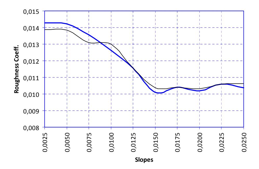
Figure 2. The relation of the base slope and the roughness coefficients of the gutter
Table 3. Computation of the Manning roughness coefficients n using the average flow rate
| b = 12 cm | Q = | 689,5 | y = 1,5 m /s c | |||
|---|---|---|---|---|---|---|
| S | y | A | P | R | n | State of |
| (cm/cm) | (cm) | (cm2 ) | (cm) | (cm) | Flow | |
| 0,0025 | 2,40 | 28,80 | 16,80 | 1,714 | 0,0139 | sub-critical |
| 0,0050 | 1,90 | 22,80 | 15,80 | 1,443 | 0,0139 | sub-critical |
| 0,0075 | 1,60 | 19,20 | 15,20 | 1,263 | 0,0131 | sub-critical |
| 0,0100 | 1,45 | 17,40 | 14,90 | 1,168 | 0,0130 | super-critical |
| 0,0125 | 1,25 | 15,00 | 14,50 | 1,034 | 0,0115 | super-critical |
| 0,0150 | 1,10 | 13,20 | 14,20 | 0,930 | 0,0104 | super-critical |
| 0,0175 | 1,05 | 12,60 | 14,10 | 0,894 | 0,0104 | super-critical |
| 0,0200 | 1,00 | 12,00 | 14,00 | 0,857 | 0,0103 | super-critical |
| 0,0225 | 0,98 | 11,76 | 13,96 | 0,842 | 0,0106 | super-critical |
| 0,0250 | 0,95 | 11,40 | 13,90 | 0,820 | 0,0106 | super-critical |
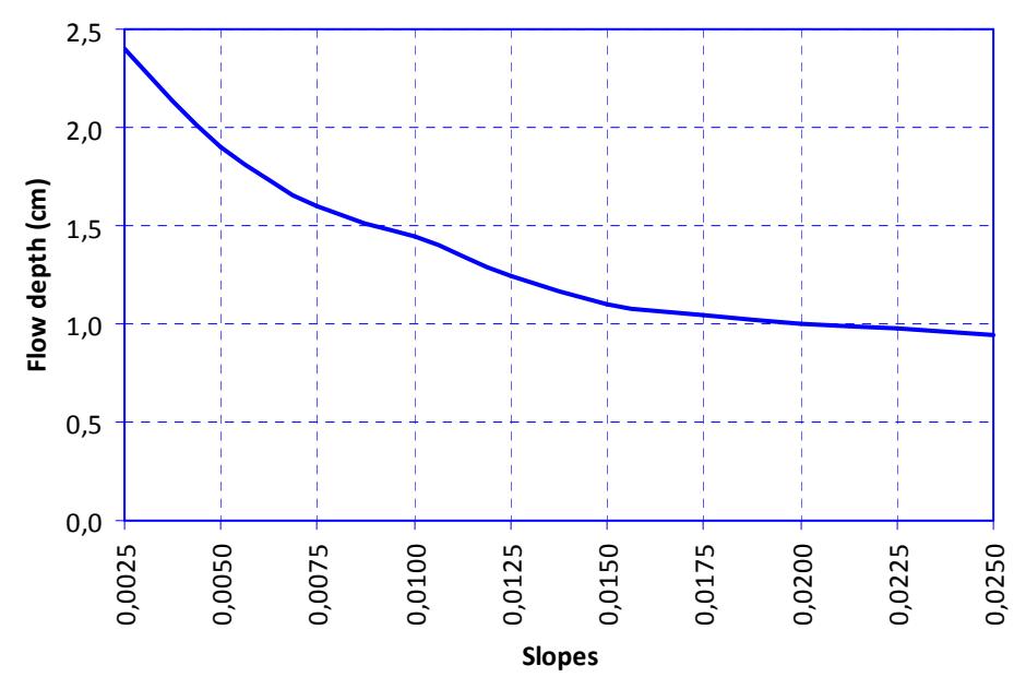
Figure 3. The gutter slope and flow depth relation
The use of the total average flow rate also has the same trend as that of partial average flow. Their discrepancies are at the mild slopes; the roughness coefficients obtained using the total average flows are smaller than those obtained using the partial one. Overall, their discrepancies can be ignored. The values of the roughness coefficient for the PVC gutter ranging between 0.010 to 0.014. The use in the normal condition, the coefficient is probably 0,011, the base slope is over 0,0125, and the flow is at the super-critical condition. The present roughness coefficients for the PVC gutter are slightly higher than the roughness coefficient for the PVC pipe as reported by Gribbin (2007) with range of 0,007 to 0,011. This variation is probably caused by the Manning equation was not derived from fundamental fluid-mechanic principles, nor was established by rigorous statistical analysis (Dingman, 2009).
The increase of the base slope S from 0.0025 becoming 0.0250 causes the flow depth drops significantly to 40 % as shown in Figure 3. The optimal gutter slope is at the rate of 0.0015, in which the water depth decreases to 48 %. At this slope, the roughness coefficient is at the stable condition.
6. Conclusions
1. The values of the roughness coefficient for the Manning formula for PVC (Polyvinyl Chloride) gutters are successfully determined with range of 0.010 to 0.014.
- 2. At the typical condition, the coefficient is probably 0.011 with the slope rate over 5 cm / 4 m. The optimal gutter slope is 6 cm / 4 m, in which the flow depth drops 52 %.
- 3. For gutters with poor maintenance cause the velocity slower, so the use of highest coefficient is better, say 0.014.
7. Recommendations
In the present study, it only uses a single PVC gutter with a rectangular shape from a specific brand. For the next studies, it is recommended to use PVC gutters with other shapes from varying brands.