
D. M. Priyantha Wedagama
Department of Civil Engineering, Faculty of Engineering, Udayana University, Bukit Jimbaran – Bali 80361 E-mail: priyantha.wedagama@gmail.com
Abstrak
Penelitian ini bertujuan untuk menyusun model-model distribusi time headway untuk analisis kinerja keselamatan lalu lintas dan kapasitas ruas jalan yang lalu lintasnya didominasi oleh sepeda motor di kota Denpasar, Bali. Tiga ruas jalan yang digunakan sebagai studi kasus adalah Jl. Hayam Wuruk, Jl.Hang Tuah, dan Jl. Padma. Analisis data menunjukkan bahwa antara 55%-80% pengendara kendaraan bermotor di Denpasar saat jam puncak pagi dan malam tidak memperhatikan jarak aman dengan kendaraan di depannya. Dari hasil penelitian ini diperoleh bahwa model distribusi lognormal terbaik untuk pemodelan data time headway saat jam sibuk pagi sementara model Weibull (3P) atau distribusi Pearson III untuk jam sibuk malam. Kapasitas ruas jalan untuk lalu lintas campuran yang didominasi oleh sepeda motor sangat dipengaruhi oleh perilaku pengendara kendaraan bermotor saat menjaga jarak aman dengan kendaraan di depannya. Kapasitas ruas jalan teoritis untuk Jl. Hayam Wuruk, Jl. Hang Tuah dan Jl. Padma adalah berturut-turut 3.186 kendaraan / jam, 3.077 kendaraan / jam dan 1.935 kendaraan / jam.
Kata-kata Kunci: Time headway, lalu lintas yang didominasi sepeda motor, keselamatan lalu lintas, kapasitas jalan.
1. Introduction
Most of traffic theories used in developing countries including Indonesia are adopted from developed countries including the USA, the UK and Australia (Minh, et al., 2005). These theories are based on homogeneous traffic dominated by light vehicles. In addition, Indonesian Highway Capacity Manual uses light vehicles as standards reference to determine the road capacity (Department of Public Works, 1997). Motorcycles however, are used by the vast majority of motorists in Indonesia for multipurpose trips. For instance, in Bali Province more than 85% of mode shares are motorcycles (Central Statistics Agency of Bali Province, 2013). As the results, the current road capacity models used in Indonesia, may not reflect the real condition of mixed traffic predominantly motorcycles.
The determination of transportation system variables consisting road capacity, level of road service and road safety are theoretically influenced by time headway, that is a time difference between the arrival of the moving vehicles. Road capacity is determined by the minimum value and distribution of time headways (Tiwari, 2000). In addition, traffic volumes and road capacity are examined on the assumption that vehicles moved and stopped consistently on road lanes (lane discipline). For mixed traffic however, determining the ideal capacity based on lane discipline may not be very precise (Tiwari, 2000).
Under such circumstances, a study on time headway for a typical mixed traffic is considered important to be carried out. In a past study (Sukowati, 2004), toll roads in Central Java are used as the case study while motorcycles certainly were not included in the analysis. Given the fact that motorcycle traffic dominates in Indonesia, this study continues the idea of such a previous study (Sukowati, 2004) in which analysing road capacity based on time headway models.
This study however, uses road traffics in Denpasar-Bali as the case study area to analyse time headway distributions in mixed traffic predominantly motorcycle. Time headway data can also be used to conduct a preliminary traffic safety analysis in terms of motorists' behaviours to keep safe (recommended) distances to the vehicles in front. This study therefore aims to develop time headway distribution models of motorcycle-dominated traffic to analyse traffic safety performance and road link capacity of single carriageways in Denpasar, Bali.
2. Literature Review
2.1 Time headway distribution models
Time headway distributions have long been studied to estimate road capacity and analyse road safety on a microscopic simulation (Al-Ghamdi, 2001). For instance, a study on time headway at signalised junctions on suburban arterial road has been conducted in South Korea (Janga, et al., 2011). The study showed that traffic volume turned out to have no effect on time headway. In addition, more influential factors at signalised junctions are that road flatness and the signal phase (Janga, et al., 2011). A previous study using California as the case study area showed that there have been differences between time headway of heavy and light vehicles on congested roads (Moridpour, 2014). This is because of the differences on driving behaviours among these drivers. Meanwhile, another past study conducted in Venice, Italy showed that the influencing factors of time headway distribution are traffic flows and their compositions especially the percentage of heavy vehicles (Rossi, et al., 2014). That previous study also found that Gamma-GQM distribution significantly explaining the effect of time headway distribution for all traffic conditions and traffic compositions.
The more traffic flows diverge, the more time headway varies. Time headway distributions for low traffic volumes are random because of the interaction among small vehicles. Time headway distributions for high and medium traffic volumes are constant and combination between random and constant respectively. Meanwhile, negative exponential distribution is the corresponding distributions for random traffic conditions and Normal and Pearson Type III distributions are best fitted to model mixed and constant time headways respectively (Sukowati, 2004). Another past study conducted on freeways in Riyadh showing that gamma and shifted exponential distributions fitted to model time headway for low and medium traffic flow respectively while Erlang distribution fitted to model high traffic flows (Al-Ghamdi, 2001). In addition, gamma distributions fitted to model traffic flows in between 600 and 1.200 vehicles/hour on arterial roads. The non-normal distributions considered in this study are:
a. Pearson III distribution model
Pearson III distribution model often called Gamma distribution with three parameters is determined as follows (Luttinen, 1996):
\[f(t \mid \tau, \beta, \alpha) = \frac{\beta^{\alpha} (t - \tau)^{\alpha - 1}}{\Gamma(\alpha)} e^{-\beta t}\] (1)
\[\Gamma(x) = \int_{0}^{\infty} y^{x-1} e^{-y} dy\] (2)
is a Gamma function and a generalization of the factorial function:
\[(x-1)! = \Gamma(x) \tag{3}\]
The distribution function consists location (\(\tau\))scale \((\beta)\) and shape \((\alpha)\) parameters.
b. Lognormal distribution model
Lognormal distribution model is determined by Pearson Type III density function and expressed as follows:
\[f(X) = \frac{1}{(X)(S)(\sqrt{2\pi})} \cdot e^{\left\{-\frac{1}{2} \left(\frac{\log(X) - (\bar{X})}{S}\right)^{2}\right\}}\](4)
where:
= Probability of lognormal distribution f(X)for the observed value of X
X Observed values
The logarithmic average of X, usually \(\overline{X}\)determined with its geometric value
S Standard deviation of logarithmic value of X
Lognormal with 3 parameters (3P) is equal to a lognormal distribution of two parameters, except that the lower limit of the additional parameter \(\beta\) is not
\[f(X) = \frac{1}{\ln(X - \beta)\sqrt{2\pi}} e^{-\frac{1}{2}\left(\frac{\ln(X - \beta) - \mu n}{\sigma n}\right)}\] (5)
where:
= Probability of lognormal distribution f(X)for the observed value of X
X = Continuous random variable
= Lower limit parameter XB
c. Weibull distribution model with 3 parameters
The probability density function (pdf) and the cumulative distribution function (cdf) of a Weibull random variable are expressed as follows (Teimouri and Gupta, 2013):
and Gupta, 2013):
\[fx(x) = \frac{\alpha}{\beta} \left( \frac{x - \mu}{\beta} \right)^{\alpha - 1} e^{-\left( \frac{x - \mu}{\beta} \right)^{\alpha}}\]
(6)
And
Figure 6. Find \[Fx(x) = 1 = e^{-\left(\frac{x-\mu}{\beta}\right)^{\alpha}}\] (7)
These equations should satisfy \(x > \mu\), \(\alpha > 0\), and \(\beta > 0\). The three parameters consist of shape \((\alpha)\), scale \((\beta)\) and location (µ) parameters. The stages to validate time headway distribution model are as follows:
- a. The number of traffic data collected should be statistically sufficient from each location while the minimum increasing traffic is between 100 and 200 vehicles per hour.
- b. As the substitute of Kolmogorov-Smirnov, Anderson-Darling and other non-parametric models chi-square test method alternatively, can be employed to test statistical distribution models. The chi-square test is expressed as follows.
\[\chi^{2}_{count} = \sum_{i=1}^{n} \frac{(f_{o} - f_{t})^{2}}{f_{t}}\] (8)
Observed data \(f_o\)
\(f_t\)Theoretical data
Chi-square count values
Chi-square (k<sup>2</sup>) method is used to determine the suitability between the theoretical (t) and empirical/ observed (o) data. Tests were carried out by constructing hypotheses as follows:
- a. \(H_0\) (hypothesis null): \(f_t = f_0\),
- b. \(H_a\) (hypothesis alternative): \(f_t \neq f_o\),
- c. The hypothesis is accepted if the \(k_{count} \le k_{table}\),
- d. The hypothesis is rejected if the \(k_{count} > k_{table}\).
2.2 Road capacity
Time headway is defined as the time between successive vehicles and measured to/from the front/rear bumper of the vehicles that passing a certain point on the road (Sukowati, 2004; Al-Ghamdi, 2001; Janga, et al., 2011; Moridpour, 2014).
\[\begin{array}{lcl} h_m & = & \sum h_p / \, n & (second/vehicle) \\ q & = & n/T = 1 \, / \, h_m & (vehicle/second) \\ q & = & 3600 \, / \, h_m & (vehicles/hour) \end{array}\] where:
\(h_p\)= Time headway (second/vehicle)
= Capacity (vehicles/hour) q
\(h_{\rm m}\)= Average time headway (second/vehicle)
= All vehicles passing a certain point during T period.
Road link capacity is determined with statistics descriptive methods by calculating mean, median, mode and the distribution percentile of time headway (Sukowati, 2004). These mean, median and mode values were calculated with empirical dan theoretical data to cope with the differences in before and after distribution modelling. The capacity can be determined by including various time headway values. By comparing each of statistics descriptive group, the highest value is considered as the ideal capacity. The percentile value is defined as a measure to indicate a percentage value below a set of data. For example, the 20<sup>th</sup> percentile is a value or score that is below 20% of observed data.
3. Case Study Area and Data Descriptions
Road segments on single carriageways (two-lane twoway undivided) of Jl. Hayam Wuruk, Jl. Hang Tuah and Jl. Padma in Denpasar are used as the case study as shown in Table 1. These segments are selected because they have high proportion of motorcycles that representing mixed traffic. In addition, these segments have low side frictions such as no on-street parking, few numbers of crossing pedestrians, non-motorised transport and exit/entry vehicles to/from the frontage.
Table 1. Road segment locations
| Jl. Hayam Wuruk | Jl. Hang Tuah | Jl. Padma | ||
|---|---|---|---|---|
| 200 m to the south of petrol station and 250 m to the north of Renon roundabout | 250 m to the west of signalised junction of Jl. Hang Tuah-Jl. Sedap Malam | Situated in Banjar Saba, the north side of the road is rice fields. | ||
Traffic data includes traffic volume and speed of each vehicle consisting motorcycles, heavy and light vehicles and time headway of pairs of vehicles. Traffic data is collected by marking reference lines on the road. Video cameras placed on either side of the road so as to record the vehicles across the observation point. Traffic volumes, speed and time headway were observed on May 19, 2015 from 06.00 to 18.00 hours. A vehicle width that is over 50% crossing a particular lane is included in that lane and not used in the other lane.
The hypotheses were constructed to express the distribution models and examined with chi-square method. Time headway distribution model are subsequently developed to determine the road capacity. Time headway data is grouped into 15 minutes interval. At each interval, the data is separated according to the arrival of pair of vehicles including:
- a. pairs of motorcycles (MCs) and light vehicles (LVs)
- b. pairs of light vehicles (LVs) and motorcycles (MCs)
- c. pairs of motorcycles (MCs) and motorcycles (MCs)
- pairs of heavy vehicles (HVs) and light vehicles (LVs)
- e. pairs of light vehicles (LVs) and heavy vehicles (HVs)
- f. pairs of heavy vehicles (HVs) and heavy vehicles (HVs) and,
- g. pairs of light vehicles (LVs) and light vehicles (LVs).
Samples used to calculate time headway were examined using criteria as follows (Sukowati, 2004):
- a. Pair of vehicles should be unobstructed by another vehicle when the front wheel passes the observation
- b. The recorded time headway is based on successive pairs of vehicles. Travel time recorded is for the leading vehicle;
- The maximum traffic volume for fifteen minutes interval is calculated and used to determine time headway distribution model and;
- d. Travel time for overtaking vehicle on the observation point is not recorded.
Table 2 shows traffic volumes at peak hours for all road segments. They are more than 1800 vehicles/hour and considered as high traffic volume. Motorcycle proportion for all segments is more than 67%, with the highest percentage was 90% in the morning peak hours at Jl. Padma. Among these three road segments, the highest volume of motorcycles (but having the lowest percentage compared to those on the other two segments) occurred on Jl. Hang Tuah. Meanwhile the largest percentage of motorcycles occurred on Jl. Padma, despite the volumes are less than those on Jl. Hang Tuah.
Table 3 shows average time headways data for pairs of different vehicle types. In theory, by using a standard of driving skills training program, two (2) seconds is the minimum safe value for time headway or safe following between a pair of vehicles (Abtahi, 2011). Interestingly, most pairs of MC-HV, LV-HV and HV-HV for all road segments kept their time headways more than two (2) seconds. This gives an indication that on the average most motorcyclists, car and truck/bus drivers paid attention to traffic safety while riding or driving behind heavy vehicles (trucks and buses). On the other hand, the pairs of MC and MC, MC and LV, LV and MC, and HV and MC for all road segments are less than two (2) seconds. These time headways are apparently below the safe limit. This indicates that on the average all motorcyclists, car and truck drivers paid less attention to traffic safety while riding or driving behind motorcycles. These occurrences are further analysed with the development of time headway models.
4. Model Development
Chi Square method is used to test the normality of the empirical data distributions. Table 4 shows that time headway distributions for these three road segments do not follow normal distribution (\(\chi^2\) sample > \(\chi^2\) table). As the results, non-normal distributions are examined accordingly.
The models are consequently calibrated with chisquare test producing the suitability of non-normal distribution which indicated with goodness of fit as shown in Table 5. The appropriate distribution is selected with the minimum \(\chi^2\) values.
Table 2. Traffic volume and speed
| NO | Road | Peak Hour(s) | Traffic F | Traffic Flow (vehicles/hour) | ||||||
|---|---|---|---|---|---|---|---|---|---|---|
| Links | . 00 | K Tiour(o) | MC (%) | LV (%) | HV (%) | МС | LV | HV | ||
| 4 | Jl. Hang | Morning | 06.45 - 07.45 | 5314 (76.7%) | 1530 (22.1%) | 83 (1.2%) | 43.4 | 40.4 | 37 | |
| ı | Tuah | Evening | 16.00 - 17.00 | 4436 (67.6%) | 2035 (31.0%) | 92 (1.4%) | 41 | 35.3 | 30.7 | |
| 2 | Jl. Hayam | Morning | 07.15 - 08.15 | 2212 (81.8%) | 479 (17.7%) | 13 (0.5%) | 44.7 | 45.3 | 67 | |
| 2 | Wuruk | Evening | 14.45 - 15.45 | 2420 (78.7%) | 644 (20.9%) | 11 (0.4%) | 37.6 | 38.6 | 59.3 | |
| 2 | II. Dadwa | Morning | 07.15 - 08.15 | 3724 (90.4%) | 358 (8.7%) | 37 (0.9%) | 39.1 | 31.8 | 46.5 | |
| 3 J | Jl. Padma | Evening | 16.45 - 17.45 | 3747 (87.0 %) | 540 (12.5%) | 20 (0.5%) | 35.3 | 31.2 | 51.3 | |
Where:
MC = Motorcycle; LV = Light vehicle; HV = Heavy vehicle
Table 3. Time headway data
| No | Road | Peak Hour - | Average Time Headway (sec) | rage T dway (: | Average Time Headway (sec) | ||||||||
|---|---|---|---|---|---|---|---|---|---|---|---|---|---|
| Links | MC- MC | MC- LV | MC- HV | LV- MC | LV- LV | LV- HV | HV- MC | HV- LV | HV- HV | ||||
| 1 | JI. Hang | Morning | 06.45 - 07.45 | 0.97 | 1.74 | 3.60 | 1.58 | 2.26 | 3.43 | 1.34 | 3.64 | 4.84 | |
| • | Tuah | Evening | 16.00 – 17.00 | 0.99 | 1.81 | 3.37 | 1.55 | 2.32 | 3.55 | 1.52 | 3.62 | 4.38 | |
| 2 | JI. Hayam | Morning | 07.15 – 08.15 | 1.23 | 1.79 | 2.04 | 1.62 | 2.03 | 3.56 | 1.79 | 3.31 | N/A | |
| 2 | Wuruk | Evening | 14.45 – 15.45 | 1.06 | 1.65 | 2.00 | 1.41 | 2.10 | 2.84 | 1.76 | 2.39 | 4.26 | |
| 2 | JI. | Morning | 07.15 – 08.15 | 1.01 | 1.91 | 3.11 | 1.43 | 2.59 | 4.52 | 1.20 | 3.29 | 4.49 | |
| 3 | Padma | Evening | 16.45 – 17.45 | 1.42 | 2.28 | 3.04 | 1.74 | 2.82 | 3.44 | 1.39 | 3.41 | 5.12 | |
Where:
MC = Motorcycle; LV = Light vehicle; HV = Heavy vehicle
30 Jurnal Teknik Sipil
Table 4. Normal distrbution test of empirical data
| Road Links | Peak Hours | \(\chi^2\) sample | \(\chi^2\) 5%,k-2 | Description |
|---|---|---|---|---|
| Jl. Hang Tuah | Morning | 402,95 | 16,9 (k=11) | Non normal data distribution |
| Ji. Hariy Tuari | Evening | 501,58 | 16,9 (k=11) | Non normal data distribution |
| Jl. Hayam Wuruk | Morning | 860,32 | 15,5 (k=10) | Non normal data distribution |
| Evening | 676,13 | 16,9 (k=11) | Non normal data distribution | |
| Morning | 296,10 | 16,9 (k=11) | Non normal data distribution | |
| Jl. Padma | Evening | 271.40 | 18,3 (k=12) | Non normal data distribution |
Where: k = number of class interval
Table 5. Goodness of fit for non-normal distributions
| Road Links | Peak Hours | Distribution | \(\chi^2\) Statistic | Descriptions |
|---|---|---|---|---|
| Pearson III | 64.347 | |||
| Jl. Hang Tuah | Morning | Lognormal | 39.765 | Best Fit |
| Weibull (3P) | 63.479 | |||
| Pearson III | 52.498 | |||
| Jl. Hang Tuah | Evening | Lognormal | 57.350 | |
| Weibull (3P) | 40.357 | Best Fit | ||
| Pearson III | 4.157 | |||
| Jl. Hayam Wuruk | Morning | Lognormal | 3.777 | Best Fit |
| Weibull (3P) | 15.289 | |||
| Pearson III | 4.339 | Best Fit | ||
| Jl. Hayam Wuruk | Evening | Lognormal | 8.135 | |
| Weibull (3P) | 13.684 | |||
| Pearson III | 26.006 | |||
| Jl. Padma | Morning | Lognormal (3P) | 23.549 | Best Fit |
| Weibull (3P) | 38.116 | |||
| Pearson III | 33.823 | |||
| Jl. Padma | Evening | Lognormal (3P) | 42.182 | |
| Weibull (3P) | 23.240 | Best Fit |
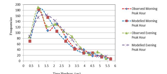
Figure 1. Frequencies of empirical and theoretical data on Jl. Hang Tuah
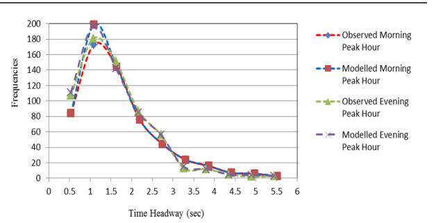
Figure 2. Frequencies of empirical and theoretical data on Jl. Hayam Wuruk
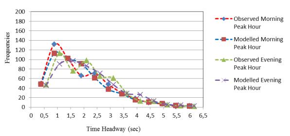
Figure 3. Frequencies of emprical and theoretical data on Jl. Padma
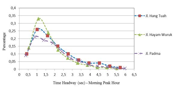
Figure 4. Probability Density Function (PDF) at morning peak hours
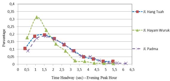
Figure 5. Probability Density Function (PDF) at evening peak hours
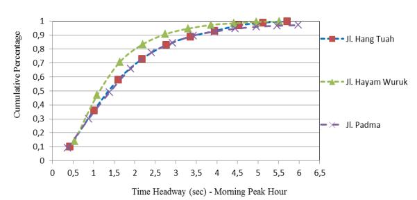
Figure 6. Cumulative Density Function (CDF) at morning peak hours
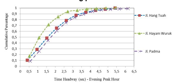
Figure 7. Cumulative Density Function (CDF) at evening peak hours
Based on Table 5, the best statistical distributions to model time headways varied among these three road segments. Lognormal distribution models are best fit to model time headways for morning peak hours on these three road segments. Meanwhile, Weibull (3P) distribution models are best fit to model time headways for evening peak hours on Jl. Hang Tuah and Jl. Padma. To model time headways for evening peak hours on Jl, Hayam Wuruk however, is best fitted with Pearson III distribution.
| Table 6. Frequencies of empirical and theoretical data | |
|---|---|
| Jl.Hang Tuah Morning Peak Hour | ||||||||||||
|---|---|---|---|---|---|---|---|---|---|---|---|---|
| Interval (seconds) | 0.13-0.71 | 0.72-1.29 | 1.30-1.88 | 1.89-2.47 | 2.48-3.06 | 3.07-3.64 | 3.65-4.23 | 4.24-4.82 | 4.83-5.41 | 5.42-6.00 | ||
| Empirical | 70 | 178 | 108 | 130 | 85 | 46 | 40 | 18 | 20 | 8 | ||
| Theoretical | 70 | 183 | 155 | 105 | 70 | 42 | 28 | 28 | 14 | 7 | ||
| Jl. Hang Tuah Evening Peak Hour | ||||||||||||
| Interval (seconds) | 0.1368 | 0.69-1.23 | 1.24-1.79 | 1.80-2.35 | 2.36-2.90 | 2.91-3.46 | 3.47-4.02 | 4.03-4.57 | 4.14-5.69 | 5.70-6.24 | ||
| Empirical | 86 | 190 | 124 | 131 | 106 | 86 | 47 | 24 | 32 | 9 | ||
| Theoretical | 88 | 154 | 163 | 142 | 109 | 75 | 42 | 29 | 17 | 17 | ||
| Jl. Hayam Wuruk Morning Peak Hour | ||||||||||||
| Interval (seconds) | 0.26-0.80 | 0.81-1.36 | 1.37-1.91 | 1.92-2.47 | 2.48-3.02 | 3.03-3.57 | 3.58-4.13 | 4.14-4.68 | 4.69-5.24 | 5.25-6.04 | ||
| Empirical | 84 | 173 | 144 | 76 | 44 | 24 | 16 | 7 | 6 | 2 | ||
| Theoretical | 84 | 199 | 144 | 76 | 44 | 24 | 16 | 7 | 6 | 3 | ||
| Jl. Hayam Wuruk Evening Peak Hour | ||||||||||||
| Interval (seconds) | 0.26-0.80 | 0.81-1.36 | 1.37-1.91 | 1.92-2.47 | 2.48-3.02 | 3.03-3.57 | 3.58-4.13 | 4.14-4.68 | 4.69-5.24 | 5.25-5.79 | ||
| Empirical | 107 | 181 | 151 | 87 | 56 | 13 | 12 | 5 | 2 | 3 | ||
| Theoretical | 111 | 197 | 142 | 85 | 56 | 15 | 12 | 5 | 4 | 3 | ||
| Jl. Padma Morning Peak Hour | ||||||||||||
| Interval (seconds) | 0.12-0.62 | 0.63-1.113 | 1.14-1.64 | 1.65-2.15 | 2.16-2.66 | 2.67-3.17 | 3.18-3.68 | 3.69-4.19 | 4.20-4.70 | 4.71-5.21 | 5.22-5.72 | 5.73-6.23 |
| Empirical | 49 | 132 | 102 | 66 | 71 | 48 | 30 | 18 | 10 | 7 | 2 | 3 |
| Theoretical | 48 | 113 | 102 | 91 | 62 | 38 | 28 | 16 | 11 | 8 | 4 | 3 |
| Jl. Padma Evening Peak Hour | ||||||||||||
| Interval (seconds) | 0.32-0.82 | 0.83-1.33 | 1.34-1.84 | 1.85-2.34 | 2.35-2.86 | 2.86-3.36 | 3.37-3.87 | 3.88-4.38 | 4.39-4.89 | 4.90-5.40 | 5.41-5.90 | 5.91-6.41 |
| Empirical | 47 | 113 | 76 | 98 | 65 | 61 | 29 | 13 | 12 | 5 | 3 | 2 |
| Theoretical | 46 | 91 | 97 | 86 | 71 | 47 | 29 | 26 | 13 | 5 | 4 | 3 |
Figures 1, 2 and 3 and Table 6 show the modelled/ theoretical and the observed/empirical frequencies of time headway. They are depicted according to best fit models on Table 5. It can be seen that graphically no significant time headway frequency differences found on the two models. Figures 4 and 5 show that the maximum time headway for morning and evening peak hours are about 1.2 seconds with the percentage of 32.5%. These both occurred on Jl. Hayam Wuruk. Figure 6 shows that about 65% of motorists at morning peak hours on Jl. Hang Tuah and Jl. Padma and nearly 80% of motorists on Jl. Hayam Wuruk experiencing theoretical time headway less than 2 seconds. In other words, between 65% and 80% of motorists during morning peak hours on these roads paid less attention to the safe distance with the vehicles in front. Figure 7 shows that between 55% and 60% of motorists at evening peak hours on Jl. Hang Tuah and Jl, Padma and about 80% of motorists on Jl. Hayam Wuruk experiencing theoretical time headway less than 2 seconds. Hence, it can be concluded that about 80% of motorists on Jl. Havam Wuruk and in between 55%-65% of motorists on Jl. Hang Tuah and Jl. Padma paid less attention to the safe distance with the vehicles in front. These such of behaviours may result in differences in road capacity and traffic safety (Abtahi, 2011).
Table 7. Central values of time headways
5. Road Capacity Determination
Road capacity is determined by theoretical distribution model that best fitted to chi-square statistical test. In order to analyse road capacity, the central values of descriptive statistics involving mean, median, mode and 90<sup>th</sup> percentile are shown in Table 7. For example, an empirical data with a value of 90<sup>th</sup> percentile is equal to 2.97 indicating that 90% of time headway data are less than 2.97 seconds. In order to determine road capacities equations (9), (10) and (11) are employed to calculate the parameters of the central values of time headways shown in Table 7.
The highest road capacity is obtained from mode values with the exception on Jl. Padma at evening peak hour for empirical data and both morning and evening peak hours for theoretical data. As the results, the road link capacities (vehicles/hour) are shown in Table 8. Theoretical time headways have the same pattern for Jl. Hayam Wuruk and Jl. Hang Tuah in which the most ideal capacity value is obtained from the mode of time headway. Meanwhile, the average value of time headway is used to determine road capacity for Jl. Padma. Morning peak hours have given the closest capacity value for empirical data on Jl. Hang Tuah and theoretical data on Jl. Hang Tuah and Jl. Hayam Wuruk.
| Empirical Data | ||||||||||||
|---|---|---|---|---|---|---|---|---|---|---|---|---|
| Road Link | Morni | ng Peak | Hour | Evening Peak Hour | ||||||||
| Road Ellik | Mean | Median | Mode | 90th percentile | Mean | Median | Mode | 90th percentile | ||||
| Jl. Hayam Wuruk | 1,68 | 1,47 | 1.43 | 2,97 | 1,58 | 1,43 | 0.95 | 2,68 | ||||
| Jl. Hang Tuah | 2.06 | 1.79 | 1.23 | 3.83 | 2.09 | 2.01 | 0.91 | 3.97 | ||||
| Jl. Padma | 1.85 | 1.55 | 1.11 | 3.35 | 2.11 | 2.10 | 2.21 | 3.59 | ||||
| Theoretical Data | ||||||||||
|---|---|---|---|---|---|---|---|---|---|---|
| Road Link | Morni | ng Peak | Hour | Evening Peak Hour | ||||||
| Rodd Link | Mean | Median | Mode | 90th percentile | Mean | Median | Mode | 90th percentile | ||
| Jl. Hayam Wuruk | 1,66 | 1,92 | 1,17 | 2,23 | 1,57 | 1,88 | 1,13 | 2,31 | ||
| Jl. Hang Tuah | 1,96 | 1,82 | 1,17 | 2,83 | 2,04 | 2,03 | 1,40 | 2,48 | ||
| Jl. Padma | 1,86 | 2,33 | 1,92 | 2,33 | 2,18 | 2,63 | 2,38 | 2,40 | ||
Table 8. Road link capacity (vehicles/hour)
| Empirical Capacity | ||||||||||
|---|---|---|---|---|---|---|---|---|---|---|
| Road Link | Morni | ng Peak | Hour | Evening Peak Hour | ||||||
| rtodd Einit | Mean | Median | Mode | 90th percentile | Mean | Median | Mode | 90th percentile | ||
| Jl. Hayam Wuruk | 2143 | 2449 | 2517 | 1212 | 2278 | 2517 | 3789 | 1343 | ||
| Jl. Hang Tuah | 1748 | 2011 | 2927 | 940 | 1722 | 1791 | 3956 | 907 | ||
| Jl. Padma | 1946 | 2323 | 3243 | 1075 | 1706 | 1714 | 1629 | 1003 | ||
| Theoreti | ool Cono | oity | ||||||||
| i neoreticai Capacity | |||||||||||||
|---|---|---|---|---|---|---|---|---|---|---|---|---|---|
| Road Link | Morning | Peak Hour | Evening Peak Hour | ||||||||||
| Rodd Ellik | Mean | Median | Mode | 90th percentile | Mean | Median | Mode | 90th percentile | |||||
| Jl. Hayam Wuruk | 2169 | 1875 | 3077 | 1614 | 2293 | 1915 | 3186 | 1558 | |||||
| Jl. Hang Tuah | 1837 | 1978 | 3077 | 1272 | 1765 | 1773 | 2571 | 1452 | |||||
| Jl. Padma | 1935 | 1545 | 1875 | 1545 | 1651 | 1369 | 1513 | 1500 | |||||
Vol. 24 No. 1 April 2017 33
Based on Table 8, theoretical road capacities for Jl. Hayam Wuruk, Jl. Hang Tuah and Jl. Padma are 3,186 vehicles/hour, 3,077 vehicles/hour, and 1,935 vehicles/ hour respectively. Theoretical capacity represents the maximum traffic flows a road section can handle while empirical capacity corresponds to the actual traffic flows crossing a section of a road. It can be seen that the highest empirical capacity values for the three segments are more than those of theoretical capacity values. This gives an initial indication that during the observation these three road segments may be overcapacity. Further investigation however, is required thoroughly to analyse this circumstance. For instance, the traffic data collected are covering weekend and two days in the weekedays.
6. Conclusions
- 1. Based on the analysis of time headway data show that between 55% -80% of motorists in Denpasar during morning and evening peak hours paid less attention to the safe distance with the vehicles in front. Parties associated with road and traffic safety therefore, should minimise this kind of behaviours on the road to reduce probability involved in traffic accidents.
- 2. The study found that the best fit distribution models for Jl. Hang Tuah and Jl. Padma during morning and evening peak hours are Lognormal and Weibull distributions with three parameters (3P) respectively. Meanwhile, the best fit distribution models for Jl. Hayam Wuruk during morning and evening peak hours are Lognormal and Pearson III distributions respectively. In other words, Lognormal distributions are the best fit for morning peak hours, while either Weibull (3P) or Pearson III distributions is suitable for the evening peak hours.
- 3. The road capacities (vehicles/hour) for motorcycledominated traffic varied as they are influenced by the motorists' behaviour in keeping safe distance with the vehicles in front. Theoretical road capacities for Jl. Hayam Wuruk, Jl. Hang Tuah and Jl. Padma are 3,186 vehicles/hour vehicles/hour, 3,077 vehicles/hour, and 1,935 vehicles/hour respectively.
- 4. Further time headway studies need to be carried out on other types of road, for instance on double carriageways, and both at signalised and unsignalised junctions. In addition, the sample size needs to be increased involving traffic during the weekend, in particular in tourists area in Bali so that the complete pictures of mixed traffic predominantly motorcycles capacities are largely captured.