
Abstrak
Ketidakpastian di dalam jaringan transportasi menjadi isu yang semakin penting di dalam dunia angkutan barang, yang secara subtantif dapat mempengaruhi komponen biaya transportasi. Sebagai parameter penting untuk membangun harga produk, variasi biaya transportasi berperan dalam mempengaruhi struktur jaringan rantai pasokan. Makalah ini kemudian mendiskusikan model supply chain network equilibrium (SCNE) dengan perilaku angkutan barang dengan mempertimbangkan variasi waktu tempuh. Cocoa SCNE model kemudian digunakan untuk mewakili rantai pasok komoditas kakao. Berbeda dengan penelitian sebelumnya, makalah ini memperhitungkan variasi arus lalu lintas dan kapasitas jalan terhadap waktu siklus pengiriman, yang secara praktis digunakan untuk memperkirakan biaya transportasi. Variasi tersebut dibangun dengan mendasarkan kepada pendekatan simulasi Monte Carlo. Akhirnya, model ini diterapkan pada jaringan rantai pasok kakao di Sulawesi untuk menyelidiki dampak variasi waktu tempuh terhadap harga kakao.
Kata-kata Kunci: Transportasi kakao, jaringan rantai pasok, stokastik, monte carlo
1. Introduction
Due to several kinds of uncertainty in transport networks (e.g., weather conditions, traffic jams, disaster, etc.), the travel time can be highly varied. Basically, the variation can be positioned in the supply side or demand side, in which the variation of travel time is resulted from the both side interactions. The variation of supply side can be illustrated by the reduction of capacity due to the crashes/incidents or disaster, as well as the traffic signal failure. In addition, the variation of demand side is depicted by the variety of traffic flow, which is a natural phenomenon in transport demand.
Since it possibly impacts the logistic cost, which is regarded as the main factor of product price formation, especially in Indonesia (The Asia Foundation, 2008; LPEM UI, 2005), such variations then convey a pressure to economic actors for providing product at reasonable cost. This fact thus motivates researches to explore the uncertainty issue in the multimode transportation, by considering the disruption issues (e.g., Bock, 2010; Huang et al., 2011; Chen and Miller-Hooks, 2012; Miller-Hooks et al., 2012), the variation of demand (e.g., Hoff et al., 2010; Meng et al., 2012) and travel time (e.g., Andersen and Christiansen, 2009; Sim et al., 2009). The latter uncertainty issue is elaborated in this paper, by investigating the impact of travel time uncertainty to the price of product. As different with the previous research, the freight cycle time is incorporated, which is rarely explored.
The freight carrier practically uses the operating cost and the cycle time to calculate the unit transport cost for moving the goods. The operating cost describes the related expense for running a freight carrier business, including the vehicle investment cost, maintenance cost and administration cost. The cycle time can be simply defined as a total time for moving the goods from the origin to the destination and return to the initial
origin, which consider the round-trip travel time, the waiting time, the loading and the unloading time. Since the cycle time is directly influenced by the variation of travel time, it is easy to understand that the transport cost, and the price of product as well, can be affected by the travel time variations. This issue is becoming more important in term of export product, which contains the long trip distance and the high risk of uncertainty. This paper then examines the impact of travel time variation to the price of cocoa bean, which is observed as the main export product of Indonesia.
As the 3rd largest cocoa producers in the world, which is mostly planted in Sulawesi Island, cocoa has a significant contribution for Indonesian economy. Even though, the logistics infrastructures potentially decrease its contribution. The poor road condition with the high risk of landslide is a growing issue relating to the logistics infrastructures in Sulawesi. This issue thus possibly affects the transport cost and cocoa price, which deteriorates the Indonesian cocoa competitiveness in global market. This paper then invokes the cocoa supply chain network equilibrium (SCNE) model for analysing the impact of travel time uncertainty to the cocoa price. The cocoa SCNE was proposed to the supply chain of cocoa, which might be typical to other agricultural product chains. The chain takes into account the behaviour of local collectors, local traders, exporters, and freight carriers (Zukhruf et. al., 2014). However, unlike the preceding research, this paper utilises the freight cycle time for estimating the unit transport cost, which is practically implemented by freight carrier company. In addition, this paper also incorporates The Monte Carlo simulation for propagating the travel time variation, and then the impact of travel time variation to the price of cocoa can be investigated.
2. Cocoa Scne Model
2.1 Model overview
Zukhruf et al. (2014) have proposed the multi-channelled cocoa SCNE model, which is developed based on the SCNE model with the behaviours of freight carriers (Yamada et al., 2009). As different with the SCNs of industrial product, the cocoa decision-makers involve local collectors, local traders, exporters, freight carriers and consumers, and it also considers the direct transaction between local traders and exporters (see Figure 1). A typical local collector is denoted by i, a typical local trader by j, a typical exporter by k, a typical demand market by l, and a typical freight carrier by h. Cocoa shipment from local collectors i to local trader j by freight carrier h is denoted by \(q_{hij}\) and \(Q^1\) is HIJ-dimensional vector of all \(q_{hij}\), where \(h = 1, \ldots, H\), i =\(1, \ldots, I\), and \(j = 1, \ldots, J\). The similar definition is stated for the shipment from local collectors i to exporter k, local trader j to exporter k, and exporter k to demand consumer l, which are denoted by \(q_{hik}\), \(q_{hjk}\), \(q_{hkl}\) and its dimensional vectors \(Q^2\), \(Q^3\), \(Q^4\) respectively. The local collectors experience the collection cost (i.e., \(f_i\)) for obtaining cocoa from farmers. They are also faced with a handling/inventory cost (i.e., \(c_i\)) for loading/ unloading, sorting, drying, packaging and storage. Facility
cost, denoted by \(g_i\), captures the expenses for operating, improving, maintaining their facilities. The transaction cost with the local trader j and exporter k are then denoted by \(c_{ij}\) and \(c_{ik}\) respectively. Transportation cost for delivering cocoa is estimated by considering the operation cost (i.e., \(w_h\)) and facility cost (i.e., \(g_h\)) of freight carrier h. For maximizing profit, local trader j and exporter k need to minimize their handling/inventory costs (i.e., \(c_j\), \(c_k\)), facility cost (i.e., \(g_j\), \(g_k\)), transaction cost (i.e., \(c_{jk}\)), and transportation cost. To make consumption decisions, the consumers at market demand l consider the cocoa prices charged by the exporters (i.e., \(c_{jk}\)). Market demand function (i.e., \(d_i(\rho^s)\)) then describes the total quantity demanded by all consumers, which depends upon the demand market prices.
The equilibrium state of cocoa supply chain network can be characterised as following variational inequality (VI) as below. However, detailed illustrations on the model are omitted in this paper, which can be discovered in Febri et al. (2014). Find a vector
\[(Q^1, Q^2, Q^3, Q^4, \gamma, \delta, \rho^4) \in R_+^{HIJ+HIK+HJK+HKL+J+K+L}\]
such that
\[\text{[rumus tidak dapat ditampilkan dengan baik — lihat PDF asli]}\]
\[\begin{split} & + \sum_{k=1}^{K} \left[ \sum_{h=1}^{H} \left( \sum_{i=1}^{I} q_{hik}^{*} + \sum_{j=1}^{J} q_{hjk}^{*} - \sum_{l=1}^{L} q_{hkl}^{*} \right) \right] \times \left[ \delta_{k} - \delta_{k}^{*} \right] \\ & + \sum_{l=1}^{L} \left[ \sum_{h=1}^{H} \sum_{k=1}^{K} q_{hkl}^{*} - d_{l} \left( \rho^{5*} \right) \right] \times \left[ \rho_{l}^{5} - \rho_{l}^{5*} \right] \\ & \forall \left( Q^{1}, Q^{2}, Q^{3}, Q^{4}, \gamma, \delta, \rho^{5} \right) \in R_{+}^{HIJ + HIK + HJK + HKL + J + K + L} \end{split}\]
Where \(R_+^{HIJ+HIK+HJK+HKL+J+K+L}\) is the nonnegative orthant in the (HIJ+HIK+HJK+HKL+J+K+L)-dimensional real space, in which the term \(\gamma_j\) and \(\delta_k\) are the Lagrange multipliers.
2.2 Travel time uncertainty model
In cocoa SCNE, the interaction between transportation network and SCN is bridged by the freight operation cost variable, which directly influence the transport cost for moving cocoa. In addition, the previous work consider the variability of travel time by involving the delay penalty cost, which is the cost incurred for avoiding substantial delay. However, this cost is not practically implemented in cocoa SCN, especially in Indonesia. Therefore this paper propose the transport cost estimation by including the cycle time, daily operation cost, and vehicle capacity, which is essentially applied by freight companies. The unit transport cost for moving cocoa is then simply calculated by taking into account the mode size and its operational time (see Eq. (2)).
\[p_{\varpi} = \frac{u_{\varpi} * t_{\varpi}(\tau, \theta)}{T s} \tag{2}\] where:
\(p_{\varpi}\): unit transport cost charged by mode \(\varpi\),
\(u_{\varpi}\): daily operation cost of mode \(\varpi\),
\(t_{\varpi}\): cycle time of mode- \(\varpi\) for transporting cocoa,
\(\tau\): random value that follow distribution \(\theta\),
\(T_{\varpi}\): daily operational hour of mode \(\varpi\),
\(s_{\varpi}\): payload capacity of mode \(\varpi\).
For capturing the actual condition, the daily operation cost is taken into account the purchasing cost for procuring the mode, the routine operation cost and the maintenance cost. The vehicle size reflects the amount of product which can be carriage by vehicle in each trip. The cycle time comprise travel time and transshipment time, which basically varies. However, in order to analyze the impact of travel time to the price, this paper assumes that the transshipment time is fixed. This unit transport is then governed the freight operation cost (i.e., \(W_h\)), which is essential part for estimating the cost for transporting cocoa.
Since cocoa is internationally consumed, the sea mode travel time is considered as the backbone of international
freight transportation mode. Equation (3) shows the travel time estimation by varying the voyage speed follows the certain distribution.
\[u_{sea} = \frac{S}{v(\tau, \theta)} \tag{3}\] where:
\(u_{sea}\): travel time of sea transportation mode,
\(\tau\): random value that follow distribution \(\theta\).
S: trip distance, v: speed (knot),
In addition, the road transportation, which play important roles in the inland transportation, is modelled by taking into account the variation of traffic flow and capacity of roads. The interaction of such variation is possibly influence the truck travel time, and subsequently impact the transport cost for distributing cocoa. Hence, the Bureau of Public Roads (BPR) function (see Eq. (4)) is then invoked for estimating the travel time at link by considering the uncertainty of traffic and road capacity.
\[u_{truck} = \sum_{a}^{A} \left( t_{a}^{0} * \left( 1 + 0.5 * \left( \frac{b_{a}(\tau, \theta) \xi}{Cap_{a}(\tau, \theta)} \right)^{1.5} \right) \right)\](4)
where:
\(u_{truck}\): travel time of truck,
\(t^0_a\): travel time of link a at free flow condition.
\(b_a\): traffic flow of link a, x: passenger car equivalent factor
\(Cap_a\): capacity of link a,
As it is implied in the Eqs. (3) and (4), the travel time are constructed by the variation of speed, capacity, and traffic flow condition. The variations are stochastically propagated within the framework of Monte Carlo simulation. Since it randomly generates by following certain distribution, which is notated by \(\tau\) and \(\theta\), the interaction of variations impacts the uncertainty of travel time for sending cocoa. Hence, it can be simply concluded that the uncertainty of travel time for distributing cocoa are fabricated in the transport network due to the variation of speed, capacity, and traffic flow.
Putting together variations in the different mode that form the unit transport cost (i.e., Eq. (2)), it can be easily investigated that the travel time variation influences the unit transport cost, which further affects the price charge by freight carrier for transporting cocoa.
3. Case Study
To investigate the effect of travel time uncertainty to the cocoa price, the model is then applied to a cocoa
SCN in Sulawesi, which is incorporated in the previous research (see Zukhruf et al., 2014). As mentioned by Syahruddin and Kalchscmidt (2012), the local collectors are mainly located in the farmers regions, and thus it is set to be positioned in the sub-district. The local traders are placed in the capital of regency/city, in which the exporters are located in the capital of province (see Figure 1 and Figure 2). To capture the actual Indonesian cocoa markets, the European region (i.e., Rotterdam), American region (i.e., New Jersey), and Asian region (i.e., Shanghai) are considered as the overseas demand markets. As different with the preceding research, this paper considers the more detail of transport network, which includes 885 road links and 3 sea port nodes. The data relating to the road conditions (e.g., capacities, speed, traffic volume, etc.) are extracted from the database of the Indonesian Integrated Road Management System (IRMS), and the seaports data are gathered from the related documents of Indonesian seaport (Indonesian Ministry of Transportation, 2012).
Local Collector Locations:
C1 – C4= Sausu, Palolo, Lara, Lambadia
Local Trader Locations:
T1 – T4= Parigi, Banawa, Masamba, Kolaka
Exporter Locations:
E1 – E3= Palu, Makassar, Kendari
Demand Market Locations:
M1 - M3= Roterdam, New jersey, Shanghai.
Figure 1. Cocoa SCN in Sulawesi
The functional forms and parameter values are then determined as follows.
\[f_i = 9720 \left( \sum_{h=1}^{2} \left( \sum_{j=1}^{4} q_{hij} + \sum_{k=1}^{3} q_{hik} \right) \right)\] (5)
\[c_i = 10 \left( \sum_{h=1}^{2} \sum_{j=1}^{4} q_{hij} + \left( \sum_{h=1}^{2} \sum_{k=1}^{3} q_{hik} \right)^{1.4} \right)^{1.6}\] (6)
\[c_{j} = 5 \left( \sum_{h=1}^{2} \sum_{i=1}^{4} q_{hij} \right)^{1.4}\] (7)
\[c_k = 40 \left( \sum_{h=1}^{2} \left( \sum_{j=1}^{4} q_{hjk} + \sum_{i=1}^{4} q_{hik} \right) \right)^{1.4}\] (8)
\[c_{ij} = 50 \left( \sum_{h=1}^{2} q_{hij} \right) \tag{9}\]
\[c_{ik} = 50 \left( \sum_{h=1}^{2} q_{hik} \right) \tag{10}\]
\[c_{jk} = 50 \left( \sum_{h=1}^{2} q_{hjk} \right) \tag{11}\]
\[c_{kl} = 50 \left( \sum_{h=1}^{2} q_{hkl} \right) \tag{12}\]
\[g_i = 20 \left( \sum_{h=1}^{2} \left( \sum_{j=1}^{4} q_{hij} + \sum_{k=1}^{3} q_{hik} \right) \right)\] (13)
\[g_j = 20\sum_{i=1}^{2}\sum_{j=1}^{4}q_{hij} \tag{14}\]
\[g_k = 20 \left( \sum_{h=1}^{2} \left( \sum_{j=1}^{4} q_{hjk} + \sum_{i=1}^{4} q_{hik} \right) \right)\] (15)
\[g_h = 20 \left( \sum_{i=1}^4 \sum_{j=1}^4 q_{hij} + \sum_{i=1}^4 \sum_{k=1}^3 q_{hik} + \sum_{j=1}^4 \sum_{k=1}^3 q_{hjk} + \sum_{k=1}^3 \sum_{l=1}^3 q_{hkl} \right)\] (16)
\[d_{l} = \begin{cases} 1.6(250 - 0.5\rho_{l}^{5}) & if \quad l = 1\\ 1.8(250 - 0.5\rho_{l}^{5}) & if \quad l = 2\\ 0.5(250 - 0.5\rho_{l}^{5}) & if \quad l = 3 \end{cases}\] (17)
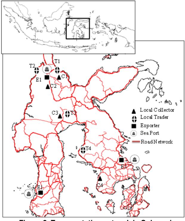
Figure 2. Transportation network in Sulawesi
4 Jurnal Teknik Sipil
Equation (5) reflects the cost for collecting cocoa from farmers, functional forms (6) – (8) show the handling cost, which is set to be non-linear. The transaction and facility cost incurred by the economic actors are formed by Eqs. (9) – (16). The cocoa demand in the international market is illustrated by Eq. (17).
For assuring the quality of model, the result of SCNE model is firstly compared to the observed data (The Asia Foundation, 2008; LPEM UI, 2005; Syahruddin and Kalchscmidt, 2012; Ali and Rukka, 2011; Yantu et. al., 2010; International Trade Center, 2011). The ratio of average logistics costs, the ratio of handling cost to total sales and the estimated ratio of transport cost to total sales for distributing cocoa from Makassar to the overseas market are then confirmed with the actual data (International Trade Center, 2011). In general, the model shows the consistent result compare to the actual data, where the ratio of average logistics costs is estimated as 10.2%, while the actual observed values as 11.7%. In addition, the ratio of handling cost to total sales is calculated as 2.7%, 1.9% and 1.9% for local collectors, local traders and exporters, respectively, while the observed value as 2.3%, 0.8% and 1.7%. The similar result is also showed by the values of overseas transport cost ratio to total sales, where the estimated value consistent with the observed data.
In order to illustrate the uncertainty of travel time, the Monte Carlo simulation is invoked for randomly generating the traffic flow and capacity. The variation in the sea mode transportation is ignored for clearly understanding the effect of travel time in the land transportation. The variation of traffic flow is then developed by considering its actual fluctuation. Since the travel time variation is assembled by its capacity and flow variation, this paper discuss three different scenarios, namely:
- Traffic flow uncertainty scenario (flow scenario),
- Assume the traffic flow is varied as it is occurred as the natural phenomena in the transportation subjects.
- Capacity uncertainty scenario (cap. scenario),
- Consider the decrement of capacity due to the landslide, which is frequently occurred in the Trans-Sulawesi road segment.
- Capacity and traffic flow uncertainty (cap-flow scenario),
- Simultaneously account the variation of capacity and traffic flow.
In the first scenario, it is assumed that the traffic flow is varied by capturing the actual fluctuation of traffic flow in Trans-Sulawesi road segment. Furthermore, the second scenario is constructed by considering the landslide event. Data recorded by the national board of disaster management (i.e., BNPB) is then utilized for identifying the critical segments, which can be listed as follows:
- Jl. Tarengge-Malili
- Jl. Mamuju- Kab. Majene
- Jl. Poros Pakaro
- Jl.Poros Kab. Barru Kab. Watangsoppeng
For illustrating the landslide events, the capacity of critical links are possibly reduced up to 100% (i.e., totally disrupted), in which its disruption probability is randomly generated by following the triangle distributions. The uncertainty scenario is then propagated by simulating 5000 times random number to obtain the variation of transportation network parameters (i.e., flow and capacity), which is thus utilised for investigating its impact to the cocoa SCN.
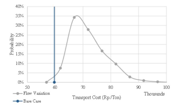
Figure 3. Transport cost variation for moving cocoa from trader to exporter (flow scenario)
Figure 3 shows the variation of transport cost due to the flow variation, in which the transport cost is varied ranging from 58,000 Rp/Ton to 100,000 Rp./Ton. This range is influenced by the variation of traffic flow, which directly impact the cycle time for moving cocoa. Since the cycle time is used for estimating the unit transport cost, the transport cost is also varied correspond to the traffic condition. As can be inferred from Figure 3, the transport cost possibly achieved the lesser cost than in the base case, although it is also possible to reach the higher cost due to the increment of traffic flow.
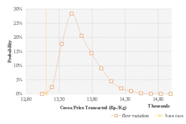
Figure 4. Cocoa price transacted between trader and exporter (flow scenario)
As the transport cost is substantially considered in the model, the change of cocoa price due to the flow variation scenario is possibly investigated. Figure 4 illustrates the change of cocoa price between Trader and Exporter, where the highest price probably increase up to 17% from base case scenario.
Table 1. Transport cost and cocoa price in the capacity uncertainty scenario
| SCN Variables | Base case | Cap. Scenario |
|---|---|---|
| Ave. Transport Cost (Rp./Ton) | ||
| Collector-Trader | 36.946 | 36.946 |
| Trader-Exporter | 59.690 | 61.798 |
| Exporter-Consumer | 47.242 | 47.242 |
| Ave. Cocoa Price Transacted (Rp./Kg) | ||
| Collector-Trader | 11.213 | 11.213 |
| Trader-Exporter | 13.102 | 13.181 |
| Exporter-Consumer | 15.070 | 15.097 |
The capacity uncertainty scenario is also elaborated for investigating the effect of land slide to cocoa SCN. Table 1 expresses the summary of cap. Scenario, where the significant increasing of transport cost is located in the transportation route that supports the trader-exporter transaction. This result is understandably corresponded to the location of critical segment, which is mainly positioned among the trade and exporter location. On contrary, the road that support the collectortrader transaction, which has low risk of landslide, does not experience the increment of cycle time, and hence the cocoa price is relatively unchanging.
However, as the small probability of total road disruption due to the landslide event, the transport cost increment is found in the relatively small amount. In line with the transport cost result, the increasing of cocoa price transacted is also found between Trader-Exporter. In addition, the increment price charged by trader sequentially affects the price in the demand market. Hence, it can be conclude that the inefficiency of transportation network potentially influence the cocoa competiveness in the global market.
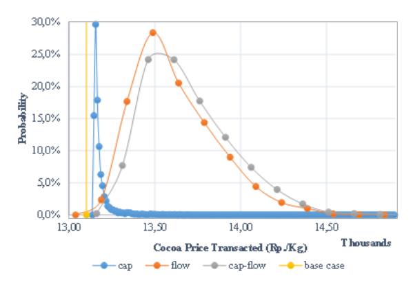
Figure 5. Cocoa price transacted between trader and exporter
The last scenario tested combines the flow and cap. scenarios. For comparing the difference among scenarios, Figure 5 shows the variation of cocoa price transacted between Trader and Exporter. As it is figured, the cap-flow scenario has a higher cocoa price than others, which is easily understood as the resultant of capacity and flow variation.
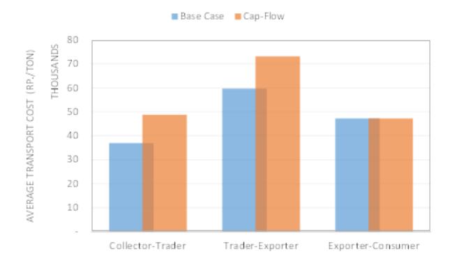
Figure 6. Average transport cost in the cap-flow scenario
However, in the actual condition, such variations firstly impact the freight carrier by changing the travel cost for moving cocoa. Therefore, the higher transport cost will initially disturb the freight carrier profit before it is affects the other economic actors. In addition, as the economic actors try to maximise his profit and the consumer has a demand function, the increment of price transacted is not bigger as it is occurred in the transport cost. (See Figures 6 and Figures 7)
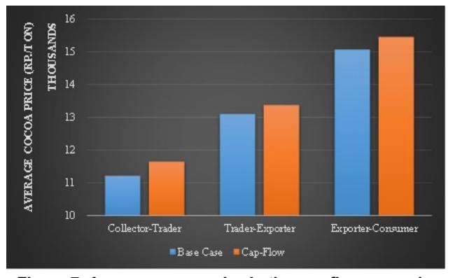
Figure 7. Average cocoa price in the cap-flow scenario
4. Conclusion
This paper models the impact of travel time uncertainty to the cocoa SCN by utilising the cocoa SCNE model with behaviour of freight carriers. As different with the existing researches, the transport cost is estimated by considering the freight cycle time, which is practically used by the freight company. Since, the cocoa price is influenced by the transport cost, the impact of travel time variation to the price then can be directly investigated. The variation of travel time is propagated using Monte Carlo simulation approach by capturing the fluctuation of traffic flow as well as the variation of road capacity for illustrating the landslide event. The model applicability is then tested using an actual cocoa SCN in Sulawesi. The numerical experiment shows that the considerable increment of travel time possibly influence the transport cost for distributing cocoa and then the cocoa price is potentially impacted.