
Abstrak
Pada praktiknya, perancangan perkerasan jalan didasarkan pada tes California Bearing Ratio (CBR). Studi ini dilakukan untuk mengetahui korelasi lokal antara tes Hand Cone Penetrometer (HCP) dan tes CBR untuk tanah dengan berat jenis yang sama, yang diambil pada beberapa titik di kota Pekanbaru, Indonesia. Berdasarkan analisis, diketahui bahwa terdapat hubungan linear, dalam skala log, antara nilai tes HCP dan CBR untuk tanah dengan berat jenis tertentu. Studi ini kemudian mendefinisikan persamaan korelasi dari HCP dan berat jenis terhadap CBR untuk korelasi lokal antara nilai HCP dan CBR. Dari hasil verifikasi persamaan, diketahui bahwa persamaan korelasi tersebut cukup akurat dan dapat digunakan untuk memprediksi nilai CBR lapangan dengan menggunakan nilai tes HCP untuk tanah inorganik. Penelitian lebih lanjut perlu dilakukan untuk mendefinisikan formula korelasi untuk tanah organic.
Kata Kunci: California bearing ratio, hand cone penetrometer, berat jenis tanah.
1. Introduction
Base (sub-grade) soil bearing capacity plays a very important role for the design of highway structure. It determines the design thickness of the pavement. The bearing capacity of the subgrade is mostly influenced by the type of soil, water content and its density. Several methods are available to determine subgrade bearing capacity such as California Bearing Ratio (CBR) test, Plate Bearing test, Dynamic Cone Penetrometer (DCP) test, and Hand Cone Penetrometer (HCP) test, which is also known as Proving Ring Penetrometer.
In Indonesia, it is a common practice to determine the subgrade soil bearing capacity for highway pavement design using CBR test measurement. This can be either the laboratory CBR test or field CBR test. Research on correlation between DCP and CBR value has been performed by Indrawan on clay sand and sand for Pekanbaru soils. The study was aimed to relate the result of DCP to CBR value, which takes into account the soil density. However, from the point of view of testing mechanism DCP test is quite different from CBR since DCP is a dynamic penetration test. On the other hand, HCP test mechanism is much closer to CBR test mechanism. HCP is a quasi-static penetration test which is also the case for CBR test. Hence, direct correlation between HCP test results to CBR value seems to be more relevant. This correlation can be based on the same soil density. This study aims to obtain direct local correlation between the two tests.
This research aims to obtain a local correlation between the results of bulk density, HCP test and CBR value. The correlation is based on the comparison HCP test results and CBR value of the same soil density.
2. Literature Review
2.1 California bearing ratio
The principle of CBR is to determine the relation between force and penetration when a cylindrical plunger with standard cross-section area is made to penetrate the soil at a given rate. At certain values of penetration the ratio of applied force to a standard force, expressed as a percentage, is defined as the California Bearing Ratio (CBR). The CBR test is an empirical test, which is used as an important criterion in pavement design. With this test, the bearing value of highway subgrade can be estimated. Several methods are described in The British Standard and American Standard for the preparation of samples for CBR test.
Basically, the CBR value describes the strength of the soil compared to the standard material. Indirectly, it also describes the relative density of the soil. Several correlations between CBR values and the results of other field measurements exist such as to results of DCP test. This has been used in practice.
2.2 Hand cone penetrometer (proving ring penetrometer)
Hand Cone Penetrometer test is relatively new. It was first developed in 1988. Hand Cone Penetrometer (HCP) testing is aimed to measure soil bearing capacity or durability of sub-grade. HCP equipment is simple to be used for soil investigation until a depth of 1 meter below ground surface. Compared to other field measurements, HCP test is relativity cheap and the test can be done quickly. Similar to other cone penetration tests such as DCP test, the results of HCP tests is in the form of cone resistance which is quasi-statically embedded into soil. The cone resistance value can be related to the density of the soil.
3. Methodology
Pekanbaru divided into thirteen sub-districts with various types of surface soil. Northern areas, clays are very dominant and in south has peat and organic soil a lot. In addition, the soil containing sand and clay is scattered in the down-town. Meanwhile, sand can be found in the south-west. Aims of this research is to obtain local correlation of field tests. Datas for verification will take in areas that represent sampling on different types of soil).
In order to obtain the correlation between HCP test results and CBR values, comparison of HCP with CBR tests results of several soil samples from Pekanbaru were performed. The HCP tests and CBR tests were performed for each soil sample from each location. Thus, the density of the soil for both tests is the same for each soil from each location. There were 40 HCP tests and 40 CBR tests performed at eight locations within the City of Pekanbaru (Figure 1).
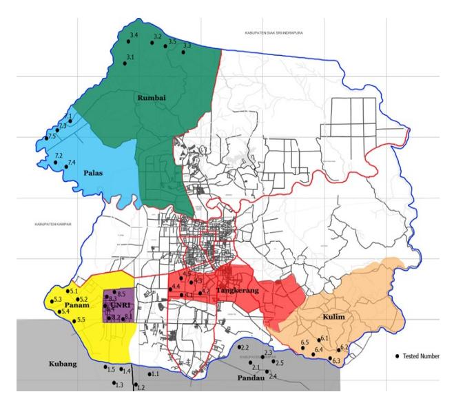
Figure 1: HCP and field CBR test
3.1 Equipment
Equipments required for field testsare a set HCP tools, field CBR tools and a CBR mould. The CBR mould was used to obtain undisturbed sample for determination of physical and mechanical properties of the soil in laboratory.
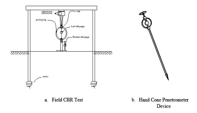
Figure 2 : Field test set-up
3.2 Testing Method
Ideally the CBR apparatus is best attached on small anchors particularly for stiff soil. However, for this case where the soil is very soft, the field CBR penetrometer system is attached on rectangular steel I beam (Universal Beam) frame with some counter weight. Thus the CBR penetrometer system is not lifted up due to CBR pressure. The HCP tests were performed simply by pressing the hand penetrometer tools into the ground.
After applying the HCP test for the eight different locations, the field CBR tools were installed very close to the HCP test locations and then the tests were performed. During the field CBR test there was no sign of lifting up on the system. This shows that the field CBR tests were performed correctly. Determination of the physical and mechanical properties of the soils, undisturbed samples were taken from each location and the tests were done in laboratory.
4. Result and Discussion
The results of this research are presented in three parts. First, the results of all performed tests are described. After that regression analysis between HCP test results and field CBR values as well as regression of HCP tests results with the density of the soils are shown. In the final part, the correlation between HCP tests results and CBR value are put forward.
The results of field tests of HCP and CBR are plotted in Figure 3. The data is plotted on a HCP against field CBR tests axes. It can be seen that there is potential relation between the two field tests results. Using the obtained data, a regression analysis was performed. From the analysis, the correlation between HCP values, bulk density and field CBR value are assessed and further discussed in a later section
4.1 Physical and mechanical properties of test samples
The test results of physical properties (i.e. natural water content (w), bulk density \((\gamma)\)) and mechanical properties (i.e. Values of field CBR (CBR), value of HCP) of the samples can be divided into four categories based on the type of soils as seen in Table 1.
Based on USCS classification system, soil properties test of samples dividing samples in 4 (four) types as fibrous peat, lean clay, sandy clay, and poorly graded sand.
For the soils which are considered as in-organic soils (sand, clay, sand-clay mixture), in general have natural water content, \(w_n\) between 10.13–56.19%, bulk density, g between 11.3–21.2 gr./cm³. Furthermore, it was recorded that the values of HCP tests on those soils were between 192.3 – 688.9 N and field CBR values between 1.01-22.43% (Table 1). It is shown that the range of the physical and mechanical properties of the soils varies considerably.
From Table 1, the properties of very loose sand at UNRI location seem to be not in the range of normal sand properties. The density of the tested samples are very low. The corresponding CBR values were only around 1 – 1.44%. The very low density might be due to the fact that the very loose sand is uniform (80 percent of sand is retained in sieve no. 200) and fully saturated. The sand substance seems to be very light that it can be observed to disperse for quite some time in water before it sinks. The low field CBR value might be due to the out spreading of the sand during the test. This will be different if the CBR test was performed in laboratory where there is a radial confining pressure from the mold.
Peat soils (organic soil), properties are significantly different compared to other soils showing that it has a significantly different characteristic compared to the other soils. (Figure 1) The minimum water content of peat is far above the maximum water content of all anorganic soils. On the other hand, the maximum values of its density, HCP, and field CBR are far below the minimum values of the an-organic soils.
Table 1. Physical and Mechanical Properties of Test Samples
| District | Kubang | Pandau | Rumbai | Tangkerang | Panam | Kulim | Palas | UNRI |
|---|---|---|---|---|---|---|---|---|
| w (%) | 180.21 | 12.05 | 13.25 | 45.33 | 43.01 | 26.28 | 10.38 | 25.09 |
| 189.26 | 10.13 | 19.14 | 37.73 | 36.09 | 16.08 | 15.46 | 28.29 | |
| 206.98 | 14.29 | 15.30 | 52.85 | 31.48 | 15.12 | 11.86 | 31.13 | |
| 225.25 | 16.18 | 14.06 | 54.14 | 39.32 | 24.06 | 14.27 | 29.17 | |
| 217.30 | 15.01 | 17.20 | 56.19 | 41.19 | 17.38 | 12.76 | 34.20 | |
| 10.72 | 20.34 | 17.44 | 14.40 | 12.21 | 14.37 | 16.89 | 12.15 | |
| 10.78 | 20.74 | 16.01 | 15.40 | 13.08 | 16.51 | 15.52 | 11.96 | |
| g (kN/m³) | 10.54 | 19.96 | 16.51 | 13.94 | 13.16 | 16.71 | 16.79 | 11.45 |
| - , | 10.53 | 19.38 | 17.79 | 13.61 | 12.85 | 14.60 | 15.69 | 11.66 |
| 10.58 | 19.74 | 15.98 | 13.33 | 12.47 | 16.24 | 16.15 | 11.06 | |
| 142.30 | 637.80 | 586.90 | 306.00 | 229.60 | 387.90 | 498.70 | 216.90 | |
| 130.70 | 688.90 | 426.30 | 494.40 | 259.30 | 468.90 | 409.30 | 208.40 | |
| HCP (N) | 123.00 | 616.50 | 498.70 | 297.40 | 267.70 | 481.70 | 477.40 | 198.10 |
| 107.00 | 599.50 | 549.10 | 288.90 | 246.60 | 396.50 | 417.80 | 200.00 | |
| 115.30 | 608.00 | 485.90 | 276.20 | 238.10 | 447.60 | 439.10 | 192.30 | |
| CBR (%) | 0.34 | 18.19 | 14.01 | 3.60 | 1.47 | 5.05 | 10.94 | 1.44 |
| 0.28 | 22.43 | 9.89 | 5.45 | 2.04 | 8.14 | 5.27 | 1.32 | |
| 0.22 | 16.19 | 10.04 | 3.37 | 2.37 | 8.79 | 8.54 | 1.14 | |
| 0.16 | 14.14 | 11.17 | 2.95 | 1.83 | 5.35 | 5.41 | 1.25 | |
| 0.19 | 15.04 | 9.07 | 2.52 | 1.69 | 6.79 | 6.49 | 1.01 | |
| USCS classify. | Fibrous peat | Lean Clay (C) | Sandy clay (S-C) | (very loose sand), SP | ||||
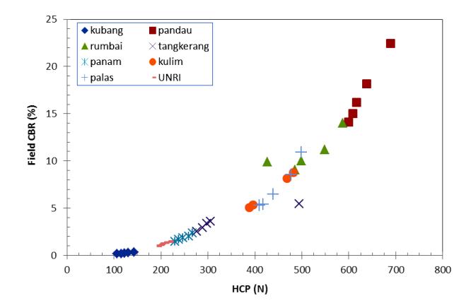
Figure 3. HCP and field CBR tests result plotted on HCP against field CBR axes
4.2 Plots of HCP-CBR and HCP-density (bulk density)
Figures 4 to 7 show the plots of HCP and density HCP and as well as plots of CBR tests values. The plots are made for each type of soils, i.e. peat, sand, clay, and sand-clay mixture. For each plots, a trend line was added to see the trend of the data.
In order to find a correlation between HCP, CBR and density values, the corresponding data is analyzed using a regression analysis. It can be seen that trend line using linier rule suits the relation between HCP and soil density relatively accurately whereas for the relation between HCP and CBR, both second polynomial and linear functions also shows relatively accurate approximation with coefficient of correlation more than 0.94. However, to simplifield linear regression was chosen. The two regression analyses (unit weight vs. HCP, CBR vs. HCP) will be combined later using Pearson's correlation method to find the correlation between unit weight, HCP test results and field CBR values.
4.3 Local Correlation between HCP Test Result and Field CBR Values
In the previous section, the plots of data between HCP and CBR as well as between HCP and soil density have been presented. In order to correlate the HCP test results to field CBR value, Pearson's correlation method is applied to both obtained power and polynomial functions for each type of soils.
On using soil density (bulk density) and the value of HCP test as variables, the following linear equation can be applied to find simple correlation between HCP and CBR on the basis of the same soil density value of soils
\[Y = C_0 + C_1 X_1 + C_2 X_2 \tag{1}\]
With
\(C_0, C_1, C_2\): constant
Y : value of field CBR (%) X<sub>1</sub> : bulk density (kN/m<sup>3</sup>)
X<sub>2</sub> : value of Hand Cone Penetrometer, HCP (N)
The volumetric unit weight,\(\gamma\) is obtained from undisturbed sample which can be done on field by measuring the weight of soil in a unit volume according to Craig's Soil Mechanics, 7th Edition (Craig, 2005) This \(\gamma\) is required to make prediction on field CBR value from the HCP test result.
The values of the constants \(C_0\), \(C_1\), and \(C_2\) for all types of soils can be solved using SPSS according to Statistics: Teory and application, \(6^{th}\) edition (Supranto, 2000) software which is based on the solution of the following matrix
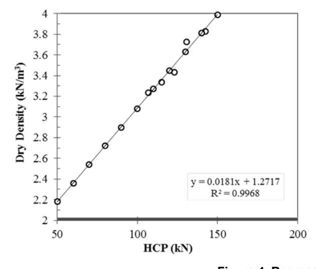
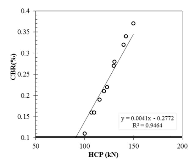
Figure 4. Regression Result for Peat
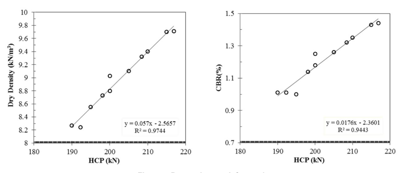
Figure 5. Regression result for sand
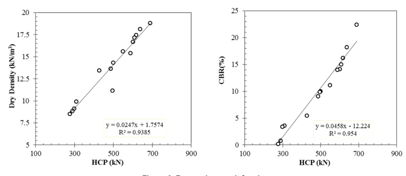
Figure 6. Regression result for clay
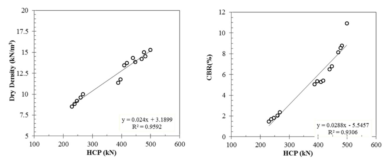
Figure 7. Regression result for sand-clay mixture
\[\begin{bmatrix} \mathbf{n} & \sum \mathbf{X}_1 & \sum \mathbf{X}_2 \\ \sum \mathbf{X}_1 & \sum (\mathbf{X}_1)^2 & \sum (\mathbf{X}_1 \mathbf{X}_2) \\ \sum \mathbf{X}_2 & \sum (\mathbf{X}_1 \mathbf{X}_2) & \sum (\mathbf{X}_2)^2 \end{bmatrix} \begin{bmatrix} \mathbf{C}_0 \\ \mathbf{C}_1 \\ \mathbf{C}_2 \end{bmatrix} = \begin{bmatrix} \sum \mathbf{Y} \\ \sum (\mathbf{X}_1 \mathbf{Y}) \\ \sum (\mathbf{X}_2 \mathbf{Y}) \end{bmatrix}\](2)
For all types of soils, the values of \(C_0\), \(C_1\), and \(C_2\) were found and presented in Table 3:
4.4 Validation of the Local Correlation Formula
For the validation of Equations 3, several prediction tests have been performed. This validation is based on different test position in each test site (on the same location), for the CBR prediction the authors use density value and HCP value to get CBR value from
Table 3. Coefficient value C<sub>0</sub>, C<sub>1</sub>, and C<sub>2</sub> for all types of tested soils
| Soil type (USCS) | C0 corr. | C0 proposed | C1 corr. | C1 proposed | C2 corr. | C2 proposed |
|---|---|---|---|---|---|---|
| Peat | -1.250 | - | 0.085 | - | 0.005 | - |
| Clay | -8.700 | -8.70 | 0.310 | 0.310 | 0.031 | 0.025 |
| Clayey Sand | -7.700 | -7.70 | 0.256 | 0.256 | 0.025 | 0.025 |
| Sand | -6.700 | -6.70 | 0.334 | 0.334 | 0.020 | 0.025 |
| All types of soils | -13.560 | *-7.25 | 0.943 | *0.25 | 0.016 | *0.025 |
*proposed for in-organic soils
For all of soils (all data is included), it was found that values of C<sub>0</sub>, C<sub>1</sub>, and C<sub>2</sub> are -13.56, 0.943, and 0.016 respectively. If the analysis of regression is performed for each types of soil separately, different constants values of C<sub>0</sub>, C<sub>1</sub>, and C<sub>2</sub> are found for each type of soils. However, comparing the results of each type of in-organic soils (sand, clay, and clay-sand mixture), the constants values of each types of soils are relatively close as can be seen in Table 3. This is not the case for organic soils (i.e. peat), the constants value for peat are significantly different from the values of in -organics soils. Since only little data are available for peat soils, more tests including consideration of the influence of peat fiber are required. It seems that the constants values are influenced by fiber content of the peat. For in-organic soils, if the average value of corresponding constant, C2 is used, the solution of C2
For in-organic soil, the local correlation formula can be written as follow:
\[Y=C_0+C_1X_1+0.025X_2\] (3a)
Substitute Y, \(X_1\), \(X_2\) with Field CBR<sub>prediction</sub>, \(\gamma\), and HCP respectly, equation (3a) can be arrangement as
Field CBR prediction = \[C_0 + C_1 \gamma + 0.025 \text{ HCP}\] 3b)
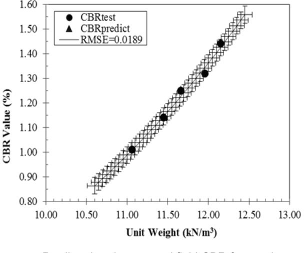
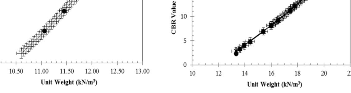
Where \(C_0\) and \(C_1\) is -6.70 and 0.334 for sand (Figure 8a), -8.70 and 0.310 for clay (Figure 8b), and -7.70 and 0.256 for sand-clay mixture (Figure 8c). HCP is the value of HCP test.
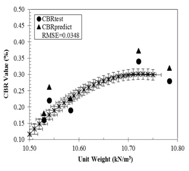
For peat soils, the value of C<sub>0</sub>,C<sub>1</sub>, and C<sub>2</sub> significantly influenced by fiber peat. The value of \(C_0\), \(C_1\), \(C_2\) is -1.250, 0.085, and 0.005 respectively (Figure 8d), however these constants need to be further tested considering fiber peat, It was difficult to find proper values for constants which might be due to the influence of fiber content of the peat.
this Equations 3 and CBR test were also perform in the same locations.
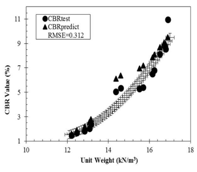
Figure 8a to Figure 8d show the comparison between predicted values of field CBR and measured field CBR values for different soil types, HCP values and soil
It can be seen from Figure 8a to Figure 8c, the predicted field CBR values give significant agreements with the measured field CBR in inorganic soils (sand, clay, sand-clay mixture). On the other hand, very poor agreements were found for peat soils. Hence, the local correlation formula is only valid for inorganic soils. For peat soils further tests and verification needs to be
Hence, by given value of C<sub>1</sub> equal to 0.25 which is the average for inorganic soils (sand, clay, sandy clay, clayey sand), the local correlation formula as stated in Equation (3) is valid for in-organic soils only and can be rewritten as below:
Field CBR prediction = \[C_0 + 0.250 \gamma + 0.025 \cdot \text{HCP}\] (4)
\[RMSE = \sqrt[2]{\frac{1}{n} \sum_{i=0}^{i=n} (CBR_{test} - CBR_{predict})^2}\] (5)
Figure 9 shows the comparison between predicted value of field CBR and measured field CBR values for different densities of in-organic soil (sand, clay, sandclay) by given value of C<sub>0</sub> from equation (4) is -7.25 which is a number from soil containing 50 % sand and 50% clay.
Figure 9 is similar with Figure 8a to Figure 8c. It can be seen from Figure 9 that the predicted field CBR value using Equation 4 and measured field CBR values give a relatively good agreement. Some small difference from the predicted and measured field CBR values may be caused by level of disturbance of sand

c. Predicted and measured field CBR for sand-clay mixture
d. Predicted and measured field CBR for peat
Figure 8: Comparison between predicted field CBR with measured field CBR for different soil types and soil densities
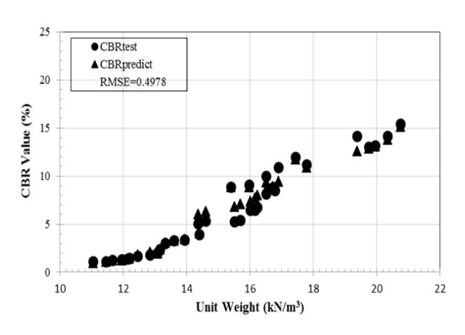
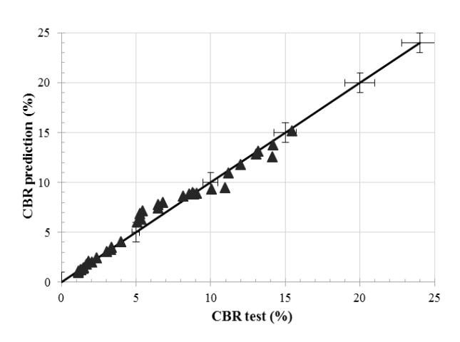
Figure 9. Predicted and measured field CBR for in-organic soil
when the tests are performed. Nevertheless, the prediction can be considered relatively accurate. Finally, equation 4 can be used to predict field CBR values from HCP value and bulk density.
5. Conclusions
This research has been performed to find local correlation between HCP test results and field CBR values. A linear regression with two variables, to find a correlation for HCP and density to CBR, has been put forward for the local correlation between the two values. Verification of the formula shows that the correlation can be used relatively accurate for predicting the field CBR values from the HCP test for in-organic soils (sand, clay and sand-clay mixture). More tests including consideration of the influence of peat fiber are required to find a good correlation. For Riau province that almost 80% of soils are peats, the formula needs to be modified and further research is needed for peat soils.