
1. Introduction
Hydrological process on the watersheds is driven by rainfall as the main input. Physical properties of the watersheds (i.e., a soil layer, topography, land uses) also affect the magnitude response of the watershed to produce run-off. Some hydrological models count, consider and involve the physical properties of the watersheds to calculate run-off produced by rainfall events. One approach elaborated by classifying watershed properties. Classification approached by selecting similar properties of the watersheds and grouping to several categories (classes). Although, nature is naturally heterogeneous or diversifies and probably it is impossible to find two watersheds that almost (100%) similar. However, some level of variability could be assumed to be similar by some criteria. Some similarities amongs watersheds may exit in the form of physical, topographic, morphometric, and hydrological properties. The similarity approach can be used to compare and to evaluate some watersheds properties. The similarity concept can also integrate into the modelling process.
Furthermore, by considering the similarity concept, hydrological process on certain watersheds can be identified. Physical properties of watersheds include form and size, river network, topography, land use, soil and geological layers. Each property probably has a strong impact on run-off production or the rainfall
process. Some researchers have been works in order to quantify some of these properties and include in the modelling process. Morphometric properties resume the quantitative relation between topography and river networks on the watershed. Interaction among morphometric, land use and soil layer determine the watershed response when rainfall event occurs. Morphometric properties can be used to conduct an analysis of ground-water resources potential and to manage the watershed. Many hydrological phenomena have a significant correlation with form and area, slope, drainage density, and other watershed properties. The amount of runoff on the watershed also depends on the structure and properties of river morphometric and catchment area. Generally, the morphometric analysis uses length, area and relief aspects of river network and watershed to derive parameter (Pande and Moharir, 2015).
Furthermore, grace the advance of GIS, Digital elevation model (DEM), hydro-informatics and remote sensing technology, more morphometrical, and other related parameters ( such as bifurcation ratio, drainage density, slope factor, soil wetness-index, etc ) can be derived automatically. Generally, the main input for morphometrical analysis is DEM. The DEM is widely available from many suppliers. For moderate resolution, the DEM can be downloaded directly from the website (for example ASTER GDEM2 available at pixel resolution 30 x 30 m can be download from https:// asterweb.jpl.nasa.gov/gdem.asp (ASTER GDEM Validation Team, 2011). More satellite vendor such as ESA (https://sentinel.esa.int/web/sentinel/home) offers sentinel image series that can derive DEM by 10m x 10m in pixel resolution. Otherwise, the DEM can also be derived by interpolation method from topographical input data, such as the work initiated by (Indarto,
Tabel 1. Morphometric parameters adopted from (Altaf, Meraj, & Romshoo, 2013; Khare et al., 2014)
| No. | Morphometric Parameters | Description | References |
|---|---|---|---|
| Linear Aspect | |||
| 1 | Stream order (U) | Hierarchical order | Strahler, 1964 |
| 2 | Stream length (Lu) | Length of the stream | Horton, 1945 |
| 3 | Mean stream length (Lsm) | Lsm = Lu/Nu where Lu=Stream length of order 'U' 1=Stream length of next lower order. 1=Stream length of next lower order. | Horton, 1945 |
| 4 | Stream length ratio (Rl) | Rl=Lu/Lu-1 where Lu=Total stream length of order 'U', Lu-Lu=Total stream length of order 'U',1=Stream length of next lower order. | Horton, 1945 |
| 5 | Bifurcation ratio (Rb) | Rb = Nu/ Nu+1; where, Nu=Total number of stream segment of order'u'; Nu+1=Number of the segment of next higher order | Schumm, 1956 |
| Relief Aspect | |||
| 6 | Basin relief (Bh) | The vertical distance between the lowest and highest points of the watershed. | Schumm,1956 |
| 7 | Relief ratio (Rh) | Rh=Bh/Lb; Where, Bh=Basin relief;Lb=Basin length | Schumn, 1956 |
| 8 | Ruggedness number (Rn) | Rn = Bh × Dd Where, Bh =Basin relief; Dd=Drainage density | Schumm, 1956 |
| Areal Aspect | |||
| 9 | Drainage density (Dd) | Dd = L/A where the L=Total length of streams; A=Area of watershed | Horton, 1945 |
| 10 | Stream frequency (Fs) | Fs = N/A where N=Total number of streams; A=Area of watershed | Horton, 1945 |
| 11 | Texture ratio (T) | T = N1/P where N1=Total number of first-order streams; P=Perimeter of watershed | Horton, 1945 |
| 12 | Form factor (Rf) | Rf=A/(Lb) 2 ;where, A=Area of watershed, Lb=Basin length | Horton, 1945 |
| 13 | Circulatory ratio (Rc) | Rc=4πA/ P2; where, A=Area of the watershed,π=3.14, P=Perimeter of watershed | Miller, 1953 |
| 14 | Elongation ratio (Re) | Re=2√(A/π)/Lb ;where, A=Area of the watershed, π=3.14, Lb=Basin length | Schumm,1956 |
| 15 | Length of overland flow (Lof) | Lof = 1/Dd*2 where, Dd=Drainage density | Horton, 1945 |
| 16 | Constant channel maintenance ( C ) | C= 1/Dd where, Dd=Drainage density | Schumm,1956 |
| 17 | Index infiltration (IF) | IF=FS x DD where, Stream frequency (Fs), Drainage density (Dd) | Horton, 1945 |
| 18 | Compactness constant (Cc) | Cc = 0.2821 x P/ A0.5 Where, A= Area, P= Basin perimeter, km | Horton, 1945 |
Wahyuningsih, Usman, & Rohman, 2008). Furthermore, The DEM is used as input to determine the watershed boundary, river network, morphometric parameters, and another indicator relevant to topography and terrain, hydrology, and soil, such as the work of (Indarto et al. 2008; Tarboton, Bras, and Rodriguez-Iturbe, 1991). This function is facilitated more detail by many of GIS and remote sensing software, such as Terrain Analysis System (TAS) (Lindsay, 2005) and the success of software named as Whitebox_GAT (Lindsay, 2016).
Table (1) lists the 18 morphometric parameters obtained from the previous study by other researchers (Khare, Mondal, & Mishra, 2014). Those parameters consist of linear, areal and relief aspect of morphometrics. Linear aspect considers only one dimension of morphometrics properties (i.e. Length ). Some examples of a linear aspect of morphometrics are stream order (U), stream length (Lu), Mean stream length (Lsm), stream length ratio (RI), and bifurcation ratio (Rb). An areal aspect of morphometric count the properties that interact between the linear dimension of the river network and the area dimension of the watershed. Some example of areal aspect of morphometric properties are : drainage density (Dd), stream frequency (Fs), Texture ratio (T), form factor (Rf), Circulation ratio (Rc), Elongation Ratio (Re), Length of overland flow (lof), Constant Channel Maintenance (C), Index infiltration (IF), Basin shape (Bs), Compactness constant (Cc). Relief aspect of morphometric determine the properties that count interaction between topography and river network. Example of relief aspect is basin relief (Bh), Relief ratio (Rh), and Ruggedness number (Rn).
Early studies initiated by (Hermingler, Kumar, & Foufoula-Georgiou, 1993; Horton, 1933; Horton & Robert, 1945); (Miller, 1953), (Schumn, 1956), and (Strahler, 1964) discussed the importance of each morphometrical parameters in relation with hydrological processes on the watershed. Further studies conducted by many researchers in India and another part of the world do the example of how morphometric parameters derived from remote sensing data or GIS Data. Some researcher use the morphometrical properties as criteria to determine the priority level for conservation (Guth, 2011), (Toth, 2013), (Gajbhiye, Mishra and Pandey, 2014), (Chandniha and Kansal, 2014), (Rai et al., 2014), (Khare et al., 2014), (Singh and Singh, 2014), (Meshram and Sharma, 2015), (Umrikar, 2016), and (Soni, 2016). The objective of this study is: (1) to quantify the variability of physical and hydrological properties of the watersheds, (2) to find the relation between physical and hydrological properties of the watersheds.
2. Methods
2.1 Study site and input data
The study was conducted in the region of East Java Province. About 45 watersheds on the regions were used for this study (Figure 1).
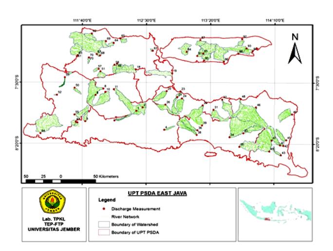
Figure 1. Location of watersheds used for this study
Watershed boundaries are determined from the DEM (Aster GDEM2) using an existing algorithm in the GIS Software. Then physical properties of the watersheds (i.e. land use, soil type, hydro-geological layers) are presented in the form of (%) areas occupied per total watershed area. The land use layer is downloaded from RBI Digital Maps of National Agency of Geospatial Information or Badan Informasi Geospasial (BIG). Other layers to describe the physical properties of the watersheds are obtained from the existing database on the Lab.TPKL (Laboratorium Teknik Pengendalian dan Konservasi Lingkungan). Furthermore, daily discharge and rainfall data obtained from an existing database. The data are collected initially from UPT Dinas PU-Pengairan Provinsi Jawa Timur. The UPT is a subadministratif unit for water resources management. Region of East Java province is composed of nine (9) UPT boundaries. The data were collected since 2004 through many schemes of cooperation including research collaboration, a student internship, undergraduate and post graduate thesis.
2.2 Statistical analysis of hydrological data
Firstly, the daily flow data from the outlets were used to derive the statistical resume of daily discharge data i.e: Maximum, Minimum, Mean, Median, Mean Daily Baseflow (MDBF), Percentile 10, 25, 33, 66, 75, 90, and 95% (P10, P25, P33, P66, P75, P90, and P95). The mean and Median is a measure of central tendency. Mean is calculated as the average of the records (sum of values/number of days). The Median is the "middle" value for the entire record: it is the value exceeded 50% of the time. For flow data, the median is usually much lower than the mean daily flow because the distribution of discharge data is negatively skewed with a lower limit of zero and no upper limit. The Percentile value is the value that is exceeded a certain percentage. For instance, the 10th percentile is the value that is exceeded by 10% of the records. Then, the statistical distribution values i.e: Standard deviation (StDev), coefficient of variance (Cv), Kurtosis (Ku), Skewness (Skew), Variability (Var), Standard deviation of the log of daily flows (S_Log), Lane Variability Index (Lane), Base Flow Index (BFI), and Flood Flow Index (FFI) were also calculated to represent hydrological properties of the daily discharge data. All of those value are calculated using the Time Series Module of the River Analysis Package (RAP) (Marsh, 2003).
The standard deviation (STDev) is a measure of how widely the values are dispersed from the mean value. For a small catchment stream, the base flow will be typically very low, with a dramatic change in discharge during a storm event. Most of the discharge thus occurs during a storm. However, most of the days are low flow. Hence the median flow is low, and the much larger event-based discharges elevate the mean flow. As a consequence, the skewness of a small catchment would be higher than that of a large catchment. Similarly, the Skewness of an unregulated stream will tend to be higher than that of a regulated stream (depending on the flow release strategy). The measure of variability (Var) used is based on the use of the median as a measure of central tendency. Variability is calculated as the range divided by the median. The user defines the range in terms of the percentile range of flows. The default setting for the range is the difference between the 10<sup>th</sup> and 90th Percentile values.
Flow data is often logged to reduce the skew, S Log is a measure of the distribution of this transformed data, as such it describes the skew of the input data (Gordon et al., 1992).
\[S_{\log} = \frac{\log(X_5) - \log(X_{95})}{3.29}\] (eq. 1)
where: X5 and X95 are the 5<sup>th</sup> and 95<sup>th</sup> percentile values respectively
The Lane's variability index (Lanes) is described as the standard deviation of the logarithms of the 5th, 15th, 25th ..., 85th and 95th percentile values. Lanes variability index is unsuitable for data sets with more than 5% zero values (i.e. 95th percentile = 0) or data sets dominated by zeros (Gordon et al., 1992).
Another indicator used in this study is an index of variability (Iv) or slope of flow duration curve (Sfdc). One approach to calculate Sfdc is by using a segment of fdc from percentile 33 (\(P_{33}\)) to percentile \(66(P_{66})\), it is assumed that this segment is relatively linear (Pallard, Castellarin and Montanari, 2009; McMillan et al., 2016) (Taylor et al., 2009). Than Sfdc is calculated using equation (2).
\[Iv = Sfdc = \frac{\ln (P_{33\%}) - \ln(P_{66\%})}{(0.66 - 0.33)}\] (eq. 2)
where:
\(S_{fdc}\) = slope of FDC,
\(Q_{33\%}\) = flow at percentile 33%, and
\(Q_{66\%}\) = flow at percentile 66%.
The steepest slope in FDC curve shows that the river is subject to high variation in flow regime. The contrary, gentle slope in FDC curve indicates that the flow regime is relatively stable from time to time (during one year). The stability of the flow regime formed by the combination of rainfall events that distributed spatially around the part of the watershed area and rainfall event that consistently occur along the year. The gentle slope of FDC also shows that the contribution of groundwater portion to the river flow is significant. An example of the use of Sfdc to study the river flow regime have been published and applied by (Castellarin, 2014). Practically, flow duration curve (FDC) analysis was calculated by Hydro-office software (Gregor, 2012) and plotted using Excel.
2.3 Statistical analysis of rainfall data
Secondly, the same analysis is also conducted for daily rainfall data. Average daily rainfall data from each watershed are then entered to River Analysis Package (RAP) to calculate several values of statistical resume and distribution. Then, monthly and annual rainfall is derived from daily rainfall data using Time Series Manager Module (TSM) in RAP (Marsh, 2004; Marsh, Kennard, Arthington, Stewardson, & Arene, 2005). Analysis of rainfall data is conducted on RAP to obtain a statistical value of rainfall data. Finally, the statistical value obtained from the analysis of daily discharge and rainfall data is then compared between watersheds.
2.4 Morphometric analysis of the watershed
The Aster GDEM2 (http://asterweb.jpl.nasa.gov/ gdem.asp) (ASTER GDEM Validation Team, 2011) was clipped by watershed boundaries to describe watershed topography. Then, a series of DEM treatment and watershed delineation was processed for each watershed. Furthermore, watersheds areas are then derived automatically from the DEM on the top of GIS using Hydrological Function. Finally, the main topographical areas of the watersheds are then determined automatically from the DEM. Topographical properties are then compared among the watersheds. Secondly, the morphometric parameters of each watershed are processed from the DEM, using. Then, 18 morphometric parameters are obtained from these processes (Table 1). Finally, morphometric parameters are compared among the watersheds.
2.5 Interpretation
Simple statistical method was used to find the possible hydrological, relationships between topographic and morphometric parameters. In this study, simple correlation based on a coefficient of determination was conducted to find the relationships: (1) among morphometric parameters, (2) among hydrological (discharge and rainfall) parameters, (3) between hydrological vs morphometric parameters. In this case, the simple statistical criteria's based on the value of standard deviation (St.Dev) and coefficient of variance (Var) were used to identify the variability. If the values of St.Dev and Coef. Var less than << 1, the existing variability is categorized as "similar", it means that a certain level of "similarity" exits. Well, it not 100% similar, because the nature is always vary at certain scale of observation. This approach justified only to classifie the same level of varibility in the same class of "similarity. Contrary, if the level of variability which measured by StDev and Coef. Var is more than >> 1; then the existing variability is categorized as "different". Furthermore, this simple criterion is used to compare both of hydro-meteorological and morphometric parameters. This definition of similarity may be vague for other scientifics field, however because in hydrology the phenomenons are always varies in space and time, the simplifaction by classyfing certain level of varibility into single class and called "similar" is probably usefull for practical reasons to handle some irregularities in hydrology.
3. Results & Discussion
3.1 Main properties of the watersheds
Table.1 summarized the main properties (i.e. area, perimeter, total stream length, and strahler stream ordering numeber) of the 45 watersheds used in this study. Size of the watershed range from 17,55 to 752,00 km² and the average of the catchment area is 170,56 km². It can be stated that all of the watersheds are categorized as small watersheds. The perimeter of the watershed ranges from 21 to 177 km. Total stream length range from 13 to 1047 km. The order of river network analysed using strahler method range from 2 to 6. The altitude value range from 0 to 3000 m above sea level.
3.2 Hydrological properties of the watersheds
3.2.1 Daily discharge data
Tabel 3 resume the statistical value of daily discharge data obtained from the watersheds. Mean daily discharge for all watersheds is recorded between 0,16 to 299,87 m<sup>3</sup>/day. Maximum daily discharge data range from 8 to 7489 m<sup>3</sup>/day. Each watershed shows the variability, in term of daily discharge data, as indicated by the value of maximum, minimum, mean, median, percentile 10, percentile 90, and MDBF (Table 3). Similar appears on Standard deviation of the log of daily flow and Lanes variability index. It's show the rate of change in daily discharge distribution and described as a standard deviation of percentiles. The discharge data is normalized by the ratio between maximum to mean discharge, minimum to mean, minimum to maximum, and standard deviation to mean discharge.
3.2.2 Daily rainfall data
Due to the limit of data availability, only rainfall data from 26 watersheds are selected, compared and visualized. Table 4, present the result of statistical analysis for averaged daily rainfall data from the watersheds. Table 4 show the values obtained for statistical resume (i.e. mean, median, standard deviation, the coefficient of variation, skewness, and maximum). The similarity appears for the value of coefficient of variation and skewness. This shows the same distribution of variability and degree of skewness of daily rainfall data. The watershed are subject to similar climatic regim thatb force the similarity in dailiy rainfall data.
Table 2. Main properties of the watersheds
| Table | 2. Main properties o | f the w | atersheds | . | |
|---|---|---|---|---|---|
| Water shed Code | Watershed Names | Area (km²) | Perimeter (km) | Stream Length (km) | Stream orde |
| 1 | Lahar-Bacem | 87,00 | 72,67 | 23,59 | 3 |
| 2 | Cubanrondo-Lebaksari | 62,00 | 38,00 | 4,05 | 4 |
| 3 | Sayang-Jabon | 45,00 | 35,00 | 3,50 | 4 |
| 4 | Sumber Ampel-Baros | 27,00 | 37,00 | 5,59 | 3 |
| 5 | Bagong-Temon | 63,00 | 50,00 | 3,40 | 4 |
| 6 | Keser-Keser | 44,00 | 34,00 | 2,70 | 4 |
| 7 | Duren Kebak | 18,00 | 21,00 | 6,92 | 3 |
| 13 | Lamong-Simoanggrok | 246,89 | 107,96 | 27,39 | 4 |
| 19 | Surabaya-Perning | 218,00 | 125,26 | 37,08 | 4 |
| 20 | Kadalpang-Bangil | 143,20 | 67,59 | 32,00 | 4 |
| 24 | rejoso | 148,90 | 62,44 | 28,00 | 5 |
| 26 | Welang-Purwodadi | 159,80 | 107,80 | 29,00 | 5 |
| 29 | Kramat-Probolinggo | 234,90 | 94,41 | 48,00 | 5 |
| 31 | Pekalen-Condong | 168,20 | 85,89 | 15,00 | 4 |
| 32 | Rondodingo-Jurangjero | 181,50 | 84,47 | 22,00 | 5 |
| 33 | Mayang | 150,00 | 80,00 | 30,00 | 4 |
| 34 | Rawatamtu | 673,00 | 177,00 | 56,00 | 5 |
| 35 | Sanenrejo | 292,00 | 94,00 | 35,00 | 5 |
| 36 | Asen-Sentul | 167,00 | 87,00 | 33,00 | 4 |
| 38 | Mujur | 137,00 | 88,80 | 34,00 | 4 |
| 39 | Wonorejo | 132,00 | 63,00 | 19,00 | 4 |
| 40 | Bajulmati | 191,00 | 74,00 | 19,00 | 5 |
| 41 | Boma Atas | 156,00 | 96,00 | 22,00 | 4 |
| 42 | Bomo Bawah- | 184,00 | 110,00 | 31,00 | 4 |
| 43 | Setail-Kradenan | 37,00 | 54,00 | 16,00 | 3 |
| 44 | 4 | ||||
| 45 | Tambong-Pakistaji Karangdoro | 99,00 | 63,00 | 6,00 26,00 | 5 |
| 3 | 514,00 | 122,00 | , | ||
| 46 | Kloposawit | 752,00 | 153,00 | 18,00 | 6 |
| 48 | Deluwang-Demung | 119,00 | 104,00 | 28,00 | 4 |
| 50 | Madiun Nambangan | 36,72 | 35,67 | 5,19 | 3 |
| 55 | Madiun Ngawi | 18,34 | 49,00 | 18,00 | 2 |
| 57 | Kedungpring- | 645,62 | 152,90 | 16,05 | 5 |
| 59 | Keang-Ngindeng | 133,04 | 70,77 | 14,40 | 4 |
| 65 70 | Bengawan Solo-CEPU Gondang-Setren | 214,00 | 83,00 | 13,11 | 5 3 |
| 70 71 | Kerjo-Pejok | 20,53 56,70 | 34,70 45,19 | 1,00 2,51 | 3 4 |
| 80 | Gembul-Merakurak | 61,67 | 44,68 | 1,47 | 4 |
| 81 | Klero-Genaharjo | 37,90 | 34,59 | 9,62 | 3 |
| 83 | Prumpung-Belikanget | 102,30 | 64,41 | 4,42 | 4 |
| 84 | Blega Telok | 160,00 | 80,29 | 18,00 | 4 |
| 85 | Kemuning-Pangilen | 271,00 | 101,00 | 7,16 | 5 |
| 86 | Samiran-Propo | 297,78 | 112,34 | 30,19 | 5 |
| 90 | Sampang | 101,55 | 63,20 | 2,40 | 3 |
| 92 | Klampok-Ambunten | 49,96 | 39,93 | 5,07 | 4 |
| max | 752,00 | 177,00 | 56,00 | 6,00 | |
| min | 18,00 | 21,00 | 1,00 | 2,00 | |
| average | 174,03 | 77,29 | 18,40 | 4,09 | |
| St. dev | 170,99 | 35,62 | 13,42 | 0,80 | |
| CV | 0,98 | 0,46 | 0,73 | 0,20 |
Table 3. Daily discharge properties
| Discharge of | on all watershe | ds | |||||
|---|---|---|---|---|---|---|---|
| Discharge (m³/S) | Max | Min | Mean | ST. Dev | CV | QualEval | |
| Maximum | 7489,00 | 8,00 | 427,44 | 1178,34 | 2,76 | different | |
| Mean | 299,87 | 0,16 | 15,30 | 46,17 | 3,02 | different | |
| Median | 125,05 | 0,09 | 7,63 | 19,60 | 2,57 | different | |
| Stdev | 384,05 | 0,24 | 23,06 | 61,90 | 2,68 | different | |
| Skewness | 10,07 | 0,87 | 2,39 | 1,58 | 0,66 | different | |
| , | Variance | -1,08 | -32,58 | -5,81 | 5,77 | -0,99 | different |
| P10 | 855,64 | 0,67 | 39,39 | 131,76 | 3,34 | different | |
| P20 | 538,00 | 0,20 | 24,34 | 82,35 | 3,38 | different | |
| , h | P30 | 324,03 | 0,16 | 15,63 | 49,48 | 3,17 | different |
| P33 | 264,00 | 0,14 | 13,21 | 40,41 | 3,06 | different | |
| . | P40 | 199,00 | 0,12 | 10,55 | 30,60 | 2,90 | different |
| P50 | 125,05 | 0,09 | 7,24 | 19,42 | 2,68 | different | |
| - | P60 | 81,78 | 0,07 | 5,23 | 13,08 | 2,50 | different |
| - | P66 | 59,98 | 0,01 | 4,23 | 10,01 | 2,37 | different |
| - | P70 | 52,88 | 0,00 | 3,84 | 8,91 | 2,32 | different |
| P80 | 40,54 | 0,00 | 3,14 | 8,22 | 2,62 | different | |
| P90 | 23,15 | 0,00 | 1,75 | 4,92 | 2,81 | different | |
| P95 | 19,90 | 0,00 | 1,36 | 3,96 | 2,92 | different | |
| V_Lane | 0,82 | 0,07 | 0,32 | 0,17 | 0,54 | Similar | |
| S_log | 0,77 | 0,07 | 0,30 | 0,16 | 0,52 | Similar | |
| Ivar (SFDC) | 13,04 | -6,83 | 1,34 | 4,21 | 3,13 | different |
Table 4. Statistical resume of daily rainfall
| Watershed Names | Mean (mm/ day) | Median (mm/day) | ST. Dev | Cv | Skewness | Maximum (mm/day) | Minimum (mm/day) |
|---|---|---|---|---|---|---|---|
| Lahan Bacem | 21,33 | 15,00 | 20,67 | 0,97 | 1,80 | 137,00 | 1,00 |
| Cuban_rondo_lebaksari | 19,86 | 14,00 | 18,65 | 0,94 | 2,22 | 149,00 | 2,00 |
| Sayang_Jabon | 20,91 | 12,00 | 22,98 | 1,10 | 1,73 | 123,00 | 1,00 |
| Bagong_temon | 21,57 | 14,00 | 20,79 | 0,96 | 1,83 | 114,00 | 2,00 |
| Kadalpang_bangil | 5,42 | 0,00 | 11,05 | 2,04 | 3,15 | 95,00 | 0,00 |
| Rejoso | 3,13 | 0,00 | 7,64 | 2,44 | 3,53 | 80,00 | 0,00 |
| Welang_purwodadi | 17,79 | 10,00 | 20,84 | 1,17 | 2,27 | 224,00 | 1,00 |
| Kramat Probolingo | 19,82 | 15,33 | 16,86 | 0,85 | 1,94 | 147,00 | 1,00 |
| Pekalen Condong | 20,51 | 17,00 | 15,47 | 0,75 | 1,62 | 125,00 | 1,00 |
| Rondodingo-Jurangjero | 22,35 | 18,33 | 16,22 | 0,73 | 1,97 | 145,00 | 1,00 |
| Mayang | 5,59 | 1,00 | 9,46 | 1,69 | 2,83 | 107,25 | 0,00 |
| Rowotamtu | 4,95 | 1,43 | 7,79 | 1,58 | 2,67 | 98,29 | 0,00 |
| Sanenrejo | 4,26 | 0,00 | 10,39 | 2,44 | 3,82 | 105,00 | 0,00 |
| Mujur | 5,47 | 1,67 | 8,87 | 1,62 | 3,52 | 124,17 | 0,00 |
| Boma_Atas | 3,15 | 0,00 | 8,37 | 2,66 | 5,24 | 145,00 | 0,00 |
| Bomo_Bawah | 4,64 | 0,00 | 9,26 | 2,00 | 3,02 | 90,50 | 0,00 |
| K.setail-kredenen | 8,34 | 3,00 | 13,75 | 1,65 | 3,05 | 125,00 | 0,00 |
| Karangdoro | 4,86 | 0,50 | 8,82 | 1,82 | 3,01 | 94,50 | 0,00 |
| Kloposawit | 4,42 | 1,00 | 7,11 | 1,61 | 3,04 | 113,94 | 0,00 |
| Deluwang | 6,78 | 0,00 | 16,26 | 2,40 | 3,17 | 147,78 | 0,00 |
| madiun-nambangan | 25,72 | 14,50 | 37,98 | 1,48 | 3,09 | 182,00 | 1,00 |
| keang-ngindeng | 20,20 | 14,00 | 17,60 | 0,87 | 1,63 | 105,00 | 1,00 |
| gondang satren | 17,81 | 10,00 | 18,45 | 1,04 | 1,79 | 90,00 | 1,00 |
| kemuning-pangilen | 20,98 | 15,00 | 19,80 | 0,94 | 1,95 | 169,00 | 1,00 |
| samiran-propo | 3,07 | 0,00 | 5,65 | 1,84 | 2,85 | 55,29 | 0,00 |
| klampok-ambunten | 26,91 | 15,00 | 33,57 | 1,25 | 2,80 | 175,00 | 1,00 |
| Max (mm/day) | 26,91 | 18,33 | 37,98 | 2,66 | 5,24 | 224,00 | 2,00 |
| Min (mm/day) | 3,07 | 0,00 | 5,65 | 0,73 | 1,62 | 55,29 | 0,00 |
| Mean (mm/day) | 13,07 | 7,41 | 15,55 | 1,49 | 2,68 | 125,64 | 0,36 |
| Standar deviation | 8,56 | 7,11 | 7,92 | 0,58 | 0,85 | 36,44 | 0,58 |
| CV | 0,66 | 0,96 | 0,51 | 0,39 | 0,32 | 0,29 | 1,62 |
3.2.3 Monthly rainfall data
It is also noted, that as part of tropical climate regions, two seasons are still distinguishable in this region (rainy and dry seasons). Rainy seasons occur from October to April and dry seasons normally occur from May to September (Indarto, Susanto, & Diniardi, 2012). The amount of rainfall received during the rainy seasons is very important because more than 70% volume of total rainfall event occurs during the rainy season. The amount of rainfall from the existing 12 months is too varied. This will influence the value of statistical resume for monthly rainfall (i.e. mean, median, standard deviation, the coefficient of variation, skewness, and maximum) as shown in Table 5.
3.2.4 Annual rainfall data
The same effect is observed in annual rainfall value (Table 6). We can note from table 5 that value of standard deviation and coefficient of variation are relatively similar in a few watersheds (i.e: Sayang-Jabon, Mayang, Rowotamtu, Keang-Ngindeng, Samiran-Propo).
3.3 Morphometrical properties of the watersheds
3.3.1 Linear aspect
Table 7 present the result of statistical analysis for the linear aspect of morphometric parameters among the 44 watersheds. Some morphometric parameters are
Table 5. Statistical resume of Monthly rainfall
| Watershed Names | Mean (mm/month) | Median (mm/month) | STDev | Cv | Skewness | Maximum (mm/month) | Minimum (mm/month |
|---|---|---|---|---|---|---|---|
| Lahan Bacem | 20,57 | 19,91 | 9,36 | 0,46 | 0,79 | 58,00 | 2,00 |
| Cuban_rondo_lebaksari | 17,53 | 17,73 | 6,85 | 0,39 | 0,05 | 31,53 | 5,00 |
| Sayang_Jabon | 17,84 | 17,80 | 9,93 | 0,56 | 0,32 | 45,00 | 1,00 |
| Bagong_temon | 21,54 | 19,90 | 10,97 | 0,51 | 1,39 | 58,33 | 3,00 |
| Kadalpang_bangil | 5,46 | 3,00 | 6,03 | 1,10 | 0,97 | 23,07 | 0,00 |
| Rejoso | 3,15 | 1,28 | 3,94 | 1,25 | 1,36 | 17,71 | 0,00 |
| Welang_purwodadi | 16,43 | 16,00 | 7,38 | 0,45 | 0,22 | 35,73 | 1,00 |
| Kramat_Probolingo | 18,46 | 18,32 | 7,12 | 0,39 | 0,32 | 40,52 | 1,00 |
| Pekalen Condong | 18,76 | 19,58 | 6,76 | 0,36 | 0,01 | 46,25 | 2,25 |
| Rondodingo-Jurangjero | 20,97 | 19,85 | 7,16 | 0,34 | 0,85 | 54,00 | 4,00 |
| Mayang | 5,61 | 4,84 | 4,80 | 0,86 | 0,67 | 19,96 | 0,00 |
| Rowotamtu | 4,97 | 4,20 | 4,48 | 0,90 | 0,83 | 22,47 | 0,00 |
| Sanenrejo | 4,27 | 2,44 | 4,61 | 1,08 | 0,96 | 18,26 | 0,00 |
| Mujur | 5,48 | 5,14 | 4,24 | 0,77 | 0,68 | 19,74 | 0,12 |
| Boma_Atas | 3,14 | 1,98 | 3,34 | 1,06 | 1,06 | 12,13 | 0,00 |
| Bomo_Bawah | 4,66 | 3,62 | 4,57 | 0,98 | 0,88 | 17,75 | 0,00 |
| K.setail-kredenen | 8,85 | 8,58 | 6,08 | 0,69 | 0,38 | 25,88 | 0,00 |
| Karangdoro | 4,87 | 3,94 | 4,36 | 0,90 | 0,61 | 16,25 | 0,00 |
| Kloposawit | 4,45 | 3,00 | 4,50 | 1,01 | 0,94 | 19,23 | 0,00 |
| Deluwang | 6,81 | 3,19 | 8,80 | 1,29 | 1,68 | 40,10 | 0,00 |
| Madiun-nambangan | 21,29 | 15,23 | 27,41 | 1,29 | 5,21 | 167,50 | 7,00 |
| Keang-ngindeng | 17,62 | 18,86 | 6,40 | 0,36 | -0,13 | 30,53 | 4,50 |
| Gondang satren | 15,15 | 13,93 | 7,68 | 0,51 | 0,24 | 30,88 | 2,50 |
| Kemuning-pangilen | 19,68 | 18,80 | 10,79 | 0,55 | 1,02 | 67,50 | 1,00 |
| Samiran-propo | 3,07 | 1,16 | 3,51 | 1,14 | 0,69 | 11,44 | 0,00 |
| Klampok-ambunten | 24,48 | 15,65 | 20,28 | 0,83 | 1,15 | 67,00 | 4,00 |
| Max (mm/month) | 24,48 | 19,91 | 27,41 | 1,29 | 5,21 | 167,50 | 7,00 |
| Min (mm/month) | 3,07 | 1,16 | 3,34 | 0,34 | -0,13 | 11,44 | 0,00 |
| Mean (mm/month) | 12,12 | 10,69 | 7,74 | 0,77 | 0,89 | 38,34 | 0,91 |
| St.Dev | 7,56 | 7,52 | 5,32 | 0,32 | 0,99 | 31,31 | 1,71 |
| CV | 0,62 | 0,70 | 0,69 | 0,42 | 1,11 | 0,82 | 1,87 |
Table 6. Statistical resume of Annual rainfall
| Watershed Names | Mean (mm/ year) | Median (mm/year) | STDev | Cv | Skewness | Maximum (mm/ year) | Minimum (mm/year) |
|---|---|---|---|---|---|---|---|
| Lahan Bacem | 22,16 | 22,17 | 4,93 | 0,22 | 0,45 | 33,91 | 14,06 |
| Cuban_rondo_lebaksari | 19,95 | 20,58 | 2,79 | 0,14 | -1,08 | 22,52 | 16,14 |
| Sayang_Jabon | 20,91 | 20,85 | 0,64 | 0,03 | 0,48 | 21,73 | 20,20 |
| Bagong_temon | 21,90 | 19,59 | 5,25 | 0,24 | 1,60 | 27,92 | 18,20 |
| Kadalpang_bangil | 5,32 | 5,79 | 2,20 | 0,41 | -0,52 | 9,36 | 1,09 |
| Rejoso | 3,10 | 3,28 | 1,24 | 0,40 | -0,68 | 5,18 | 0,00 |
| Welang_purwodadi | 18,72 | 18,34 | 4,28 | 0,23 | 1,06 | 30,16 | 12,46 |
| Kramat_Probolingo | 20,02 | 19,99 | 2,07 | 0,10 | -0,46 | 22,93 | 16,09 |
| Pekalen Condong | 20,52 | 20,36 | 2,10 | 0,10 | 0,36 | 24,29 | 17,17 |
| Rondodingo-Jurangjero | 22,57 | 22,44 | 2,13 | 0,09 | -0,02 | 25,72 | 18,72 |
| Mayang | 5,54 | 5,50 | 0,81 | 0,15 | 0,66 | 7,40 | 4,12 |
| Rowotamtu | 4,90 | 4,95 | 0,94 | 0,19 | 0,34 | 7,61 | 2,92 |
| Sanenrejo | 4,09 | 3,96 | 1,18 | 0,29 | -0,35 | 5,86 | 2,00 |
| Mujur | 5,47 | 5,65 | 1,59 | 0,29 | 0,09 | 8,05 | 3,13 |
| Boma_Atas | 2,84 | 2,96 | 2,06 | 0,73 | 0,26 | 6,75 | 0,00 |
| Bomo_Bawah | 4,64 | 4,39 | 2,83 | 0,61 | -0,05 | 8,94 | 0,00 |
| K.setail-kredenen | 9,46 | 10,22 | 3,56 | 0,38 | -0,63 | 13,74 | 1,62 |
| karangdoro | 4,86 | 5,63 | 2,17 | 0,45 | -1,63 | 6,94 | 0,00 |
| kloposawit | 4,37 | 4,43 | 1,49 | 0,34 | -2,00 | 6,65 | 0,00 |
| deluwang | 7,04 | 6,01 | 3,28 | 0,47 | 1,02 | 15,59 | 3,30 |
| madiun-nambangan | 24,90 | 17,62 | 13,93 | 0,56 | 1,71 | 40,96 | 16,11 |
| keang-ngindeng | 20,20 | 20,31 | 0,95 | 0,05 | -0,51 | 21,09 | 19,20 |
| gondang satren | 16,87 | 16,67 | 3,60 | 0,21 | 0,25 | 21,16 | 13,00 |
| kemuning-pangilen | 20,78 | 18,67 | 4,53 | 0,22 | 1,60 | 31,78 | 15,79 |
| samiran-propo | 3,07 | 3,29 | 0,82 | 0,27 | -1,37 | 3,78 | 1,90 |
| klampok-ambunten | 28,49 | 24,93 | 13,66 | 0,48 | 1,27 | 47,55 | 16,54 |
| Max (mm/year) | 28,49 | 24,93 | 13,93 | 0,73 | 1,71 | 47,55 | 20,20 |
| Min (mm/year) | 2,84 | 2,96 | 0,64 | 0,03 | -2,00 | 0,00 | 0,00 |
| Mean (mm/year) | 13,18 | 12,64 | 3,27 | 0,29 | 0,07 | 17,69 | 5,57 |
| St.Dev | 8,69 | 7,96 | 3,37 | 0,18 | 0,99 | 12,37 | 7,54 |
| CV | 0,66 | 0,63 | 1,03 | 0,61 | 13,94 | 0,70 | 1,36 |
categorized similar and others are different based on the same criteria as used to compare hydrological properties (SdDev and Coef.Var).
Table 7 shows the statistical value of linear aspect. The stream order (U) and the stream length ratio (RI) has similar values. Stream order is a branching position based on the parent river in a watershed. Forty-four watersheds located in East Java have orders between 2 to 6. Stream length ratio (RI) is the ratio of the total length of the river from the high order to the low order value. The value of RI range between 0,34 to 4,32. Low RI values indicate the low cycle rate of geomorphological changes and vice versa. The value of Bifurcation ratio (Rb), Stream Length (Lu), Mean
Stream Length (Lsm) tend to be different amongs the watersheds.
3.3.2 Relief aspect
Table 8 shows the statistical value of 44 watersheds based on the rrelief aspect parameters \((Bh,Rh \ and \ Rn)\). The three parameters of relief aspect are differents amongs watersheds. Basin relief (Bh) is defined as the result of the difference between upstream and downstream to the length of the main river. The high value of Bh shows the distance between the upstream and downstream of the river is greater and vice versa.
The ruggedness number (Rn) identifies the complexity of
Table 7. Morphometric parameter - linear aspect
| Morphometric parameter | Max | Min | Mean | St.dev | cv | Qualitative evalution |
|---|---|---|---|---|---|---|
| Stream Ordo (U) | 6 | 2 | 4,09 | 0,80 | 0,196 | Similar |
| Bifurcation ratio (Rb) | 9 | 1,28 | 2,75 | 1,71 | 0,62 | Different |
| Stream Length (Lu) | 56 | 1 | 18,40 | 13,41 | 0,72 | Different |
| Mean Stream length (Lsm) | 15,33 | 0,62 | 1,59 | 2,15 | 1,35 | Different |
| Stream length ratio (RI) | 4,321 | 0,34 | 0,98 | 0,62 | 0,63 | Similar |
Table 8. Morphometric parameters - Relief aspect
| Morphometric parameters | Max | Min | Mean | St.dev | cv | Qualitative evalution |
|---|---|---|---|---|---|---|
| Basin relief (Bh) | 3,83 | 0,061 | 1,84 | 1,16 | 0,63 | Different |
| Relief ratio (Rh) | 2,08 | 0,001 | 0,27 | 0,40 | 1,47 | Different |
| Ruggedness number (Rn) | 5,63 | 0,067 | 2,46 | 1,74 | 0,71 | Different |
the relationship between the altitude and density of the river network. The Rn value is very varying from 0,067 to 5,63. Watershed having high Rn number show higher risk of erosion. The higher value of the Relief ratio (Rh) correspond to the higher risk of sedimentation rate and vice versa.
3.3.3 Areal aspect
Table 9 shows the statistical values of 44 watersheds based on areal aspect parameters. The drainage density (Dd), stream frequency (Fs), circulation ratio (Rc), length of overland (Lof), constant channel (C) has similar values. Drainage density (Dd) shows the density of stream per area of watershed. If the value of Dd < 0,62 it is indicated that the watershed tends to have more risk of flooding and if the value of Dd > 3,10 indicate the watershed condition that more risk to drought. In table 9, the value of Dd range from 0,12 to 1,93.
Stream frequency (Fs) is an index to shows the total number of streams of all orders per unit area. Fs has been related to permeability, infiltration capacity, and relief of watersheds (Montgomery D.R. & Dietrich W.E., 1992). Further, it is noted that Fs decreases as the stream number increases. The low value of Fs indicate good vegetation coverage of watershed and more infiltration capacity (Altaf et al., 2013). The value of Fs vary from 0,5 to 6,43. The average, StDev and CV value of Fs is relatively low at majority of the watersheds. It is indicate the good vegetation cover among watersheds.
The Circulation ratio (Rc) is the opposite of elongation ratio. The higher vaue of circulation ratio (Rc) indicate the higher the rate of water flow in the watershed. In table 9, the Rc value varry between 0,03 to 0,17. The relatively low value of Rc indicate the watersheds having slow respons to flow. Small values of length of overland flow (Lof) correspond to the condition of watersheds having more steepest slopes and shorter river paths, contrary high value of Lof show the watershed condition having flatty slope and more longer river path. Lof value range from 0,062 to 1,64.
The texture ratio (T) is the total number of stream segments of all orders per perimeter of that area (Horton 1945). In the present study, texture ratio varied from 0,24 to 5,71. The lower values of texture ratio indicate that the basin is plain with lower degree of slope and low infiltration capacity. The high texture ratio illustrates the shape of a watershed that has a high slope and high infiltration capacity (Gajbhiye et al., 2014). The form factor (Rf) describes the ratio of watershed area and length of the river, the higher the value of Rf indicate the shape of the watershed becomes more rounded. Elongation ratio (Re) is the ratio between the diameter of watershed roundness to the maximum length of the watershed.
The reciprocal of the drainage density (Dd) is constant of channel maintenance (C) and signifies how much drainage area is required to maintain a unit length of channel. Low values of C is associated with weakest or very low-resistance soils, sparse vegetation and mountainous terrain, while high value of C is associated with resistance soils, vegetation and comparably plain terrain (Altaf et al., 2013). The value C is varry from 0,52 to 8,06.
3.4 Interpretation
3.4.1 Morphometric vs Morphometric properties
Table 11 shows a simple analysis using coefficient correlation to find the relation among morphometric properties. The analysis comprises all morphometric parameters from the watersheds.
It is shown that some morphometric parameters have a strong correlation to other parameters. For example: Stream length (Lu), Drainage Density (Dd), stream frequency (Fs), Texture ratio (T) are related to each other. This relationship shows a correlation between the number of surface water deposits in a watershed with the infiltration rate based on area, river network, elevation, contained assistance, and infiltration capacity.
Table 9. Morphometric parameters - Areal aspect
| Morphometric parameters | Max | Min | Mean | St.dev | CV | Quality Eval |
|---|---|---|---|---|---|---|
| Drainage density (Dd) | 1,92 | 0,12 | 1,28 | 0,31 | 0,24 | Similar |
| Stream frequency (Fs) | 6,43 | 0,50 | 1,23 | 0,85 | 0,69 | Similar |
| Texture ratio (T) | 5,71 | 0,24 | 1,57 | 1,11 | 0,70 | Different |
| Form factor (Rf) | 28,53 | 0,05 | 2,86 | 5,79 | 2,02 | Different |
| Circulation ratio (Rc) | 0,17 | 0,03 | 0,103 | 0,03 | 0,32 | Similar |
| Elongation ratio (Re) | 5,14 | 0,33 | 0,60 | 0,70 | 1,16 | Different |
| Length of overland (Lof) | 1,65 | 0,06 | 0,68 | 0,21 | 0,31 | Similar |
| Constant channel maintenant (C ) | 8,06 | 0,52 | 1,06 | 1,11 | 1,05 | Similar |
| Area (A) | 752 | 18 | 174,03 | 170,98 | 0,98 | Different |
| Perimeter (P) | 177 | 21 | 77,29 | 35,623 | 0,46 | Different |
Table 10. Morphometric parameters of watersheds
| Table 10. Morphonic | . 10 0 | ||||||||||||||||||||
|---|---|---|---|---|---|---|---|---|---|---|---|---|---|---|---|---|---|---|---|---|---|
| Watershed Names | Limier aspect | Stream Orde (U) | Bifurication ratio (Rb) | Stream Lenght (Lu) | Mean Stran lengt (Lsm) | Stream length ratio (RI) | Relief Aspect | Basien relief (Bh) | Relief ratio (Rh) | Ruggedness number (Rn) | Areal aspect | Drainage densty (Dd) | Stream freequency (Fs) | Texture ratio (T) | Form factor (R.f.) | Circulatioan ratio (Rc) | Elongation ratio (Re) | Lenght of overland (Lof) | Constant chanel (C) | Area (A) | Penimeter (P) |
| Lahar-Bacem | 3.00 | 1.54 | 23.59 | 1.58 | 0.83 | 1,53 | 0.06 | 2.40 | 1.57 | 1.04 | 0.39 | 0.16 | 0.07 | 0.67 | 0.64 | 0.64 | 87.00 | 72,67 | |||
| Cubanrondo-L ebaksari | 1 | 4,00 | 2.75 | 4.05 | 0.96 | 0.34 | 1,38 | 1.31 | 1,68 | 1 | 122 | 1.05 | 0.87 | 3,77 | 0.17 | 0.52 | 0.82 | 0,82 | 62,00 | 38,00 | |
| Sayang-Jabon | † | 4.00 | 1.77 | 3,50 | 1.08 | 0.44 | 1 | 1,64 | 0.82 | 2.39 | 1 | 1,46 | 1.00 | 0.66 | 3.67 | 0.15 | 0.44 | 0.68 | 0,68 | 45,00 | 35.00 |
| Sumber Ampel-Baros | † | 3.00 | 1,73 | 5,59 | 2.46 | 0.51 | 1 | 1,85 | 0.33 | 2.97 | 1 | 1,61 | 0.63 | 0.24 | 0.86 | 0.08 | 0.34 | 0.62 | 0.62 | 27.00 | 37.00 |
| Bagong-Tem on | † | 4.00 | 5,71 | 3.40 | 1.06 | 0.48 | 1 | 1,13 | 2.08 | 1.29 | 1 | 1.14 | 0.94 | 0.60 | 5.45 | 0.10 | 0.56 | 0.88 | 0.88 | 63.00 | 50.00 |
| Keser-Keser | + | 4.00 | 1.98 | 2,70 | 0.80 | 0.55 | 1 | 0,90 | 0.33 | 0.89 | 1 | 0.98 | 120 | 0,79 | 6.04 | 0.15 | 0.65 | 1.02 | 1.02 | 44.00 | 34.00 |
| Duren Kebak | + | 3,00 | 1,71 | 6.92 | 123 | 2,32 | 1 | 0,72 | 0.10 | 0,74 | 1 | 1.03 | 1.17 | 0,79 | 0,38 | 0,15 | 0,62 | 0.97 | 0.97 | 18.00 | 21,00 |
| + | - | - | - | + | - | - | 1 | - | - | - | - | - | - | - | - | - | |||||
| Lamong-Simoanggrok | + | 4,00 | 1,71 | 27,39 | 0,88 | 0,90 | + | 0,17 | 0,01 | 0,20 | 1 | 1,15 | 1,22 | 2,79 | 0,33 | 0,08 | 0,55 | 0,58 | 0,87 | 246,89 | 107,96 |
| Surabaya-Peming | + | 4,00 | 1,67 | 37,08 | 0,90 | 1,03 | + | 0,07 | 0,00 | 0,08 | - | 1,16 | 1,31 | 2,28 | 0,16 | 0,06 | 0,55 | 0,58 | 0,86 | 218,00 | 125,26 |
| Kadalpang-Bangil | + | 4,00 | 2,29 | 32,00 | 1,59 | 1,07 | - | 3,30 | 0,11 | 5,18 | - | 1,57 | 1,02 | 1,09 | 0,14 | 0,13 | 0,41 | 0,78 | 1,57 | 143,20 | 67,59 |
| rejoso | 4 | 5,00 | 4,22 | 28,00 | 1,32 | 0,71 | 2,72 | 0,10 | 4,43 | - | 1,63 | 0,56 | 1,17 | 0,19 | 0,15 | 0,39 | 0,82 | 1,63 | 148,90 | 62,44 | |
| Welang-Purwodadi | 4 | 5,00 | 3,21 | 29,00 | 1,17 | 0,85 | 2,27 | 0,08 | 3,20 | - | 1,41 | 1,06 | 0,81 | 0,19 | 0,06 | 0,45 | 0,71 | 1,41 | 159,80 | 107,80 | |
| Kram at-Probolinggo | 1 | 5,00 | 2,00 | 48,00 | 1,28 | 0,97 | 2,59 | 0,07 | 3,78 | 1 | 1,46 | 1,03 | 1,29 | 0,10 | 0,11 | 0,44 | 0,73 | 1,46 | 234,90 | 94,41 | |
| Pekalen-Condong | _ | 4,00 | 1,66 | 15,00 | 1,24 | 0,89 | 2,95 | 0,08 | 3,89 | 1,32 | 0,50 | 0,98 | 0,75 | 0,09 | 0,48 | 0,66 | 1,32 | 168,20 | 85,89 | ||
| Rondodingo-Jurangjero | 1 | 5,00 | 3,63 | 22,00 | 1,65 | 1,29 | 0,29 | 0,09 | 0,34 | 1,17 | 0,99 | 1,07 | 0,38 | 0,10 | 0,54 | 0,58 | 1,17 | 181,50 | 84,47 | ||
| Mayang | 4,00 | 6,26 | 30,00 | 1,46 | 1,06 | 2,61 | 0,09 | 3,89 | 1,49 | 1,06 | 1,00 | 0,17 | 0,09 | 0,43 | 0,74 | 0,67 | 150,00 | 80,00 | |||
| Rawatamtu | 5,00 | 2,43 | 56,00 | 1,39 | 1,00 | 2,74 | 0,05 | 3,78 | 1,38 | 1,00 | 1,90 | 0,21 | 0,09 | 0,46 | 0,69 | 0,73 | 673,00 | 177,00 | |||
| Sanenrejo | T | 5,00 | 1,82 | 35,00 | 0,89 | 1,16 | 1,17 | 0,03 | 1,15 | ] | 0.98 | 1,17 | 1,84 | 0.24 | 0,13 | 0,65 | 0,51 | 1,02 | 292,00 | 94,00 | |
| Asen-Sentul | 1 | 4,00 | 2,02 | 33,00 | 1,02 | 1,40 | 2,64 | 0.08 | 3,96 | 1 | 1.50 | 1.96 | 1.95 | 0,15 | 0.09 | 0,42 | 0,75 | 0,67 | 167,00 | 87,00 | |
| Mujur | † | 4.00 | 3,23 | 34,00 | 0.81 | 0,95 | 1 | 3,61 | 0,11 | 5,63 | 1 | 1,56 | 1,85 | 1,32 | 0,12 | 0,07 | 0,41 | 0,78 | 0,64 | 137,00 | 88,80 |
| Wonorejo | 1 | 4,00 | 1.77 | 19.00 | 1.42 | 1.02 | 1 | 1,63 | 0.09 | 2.35 | 1 | 1.44 | 0.98 | 1,03 | 0.37 | 0.13 | 0.44 | 0.72 | 0.69 | 132.00 | 63,00 |
| Bajulmati | 1 | 5,00 | 9.00 | 19,00 | 1,40 | 0,38 | 1 | 2.20 | 1.10 | 3,43 | 1 | 1.56 | 0.96 | 124 | 0.53 | 0,14 | 0,41 | 0,64 | 0,64 | 191,00 | 74,00 |
| Boma Atas | † | 4,00 | 2.72 | 22,00 | 1,73 | 0,61 | 1 | 3,20 | 0,15 | 4.90 | 1 | 1.53 | 1,01 | 0,82 | 0,32 | 0,07 | 0,42 | 0,65 | 0,65 | 156,00 | 96,00 |
| Bom o Bawah-Rogojampi | + | 4,00 | 2,43 | 31,00 | 1,62 | 0,64 | 1 | 3,20 | 0.10 | 4,80 | 1 | 1,50 | 0.99 | 0,84 | 0.19 | 0.06 | 0,42 | 0,67 | 0,67 | 184,00 | 110.00 |
| Setail-Kradenan | + | 3,00 | 7,50 | 16,00 | 15,33 | 0,70 | 1 | 1,50 | 0.09 | 2,89 | 1 | 1.93 | 0.95 | 0,33 | 0,19 | 0,05 | 0,42 | 0,52 | 0,52 | 37,00 | 54,00 |
| + | 4.00 | 2,33 | _ | 2.01 | 0,70 | + | 1,20 | 0,09 | 0.73 | 1 | 0.61 | 6.43 | 5,71 | 2,75 | 0.10 | 0.39 | 1.65 | 1.65 | 99.00 | _ | |
| Tambong-Pakistaji | + | _ | 6,00 | - | - | + | - | - | 1 | - | - | _ | - | - | - | - | - | - | 63,00 | ||
| Karangdoro | - | 5,00 | 2,03 | 26,00 | 1,29 | 0,50 | + | 3,20 | 0,12 | 4,45 | - | 1,39 | 1,01 | 2,10 | 0,76 | 0,14 | 0,46 | 0,72 | 0,72 | 514,00 | 122,00 |
| Kloposawit | + | 6,00 | 6,63 | 18,00 | 1,65 | 0,52 | - | 3,10 | 0,39 | 4,32 | - | 1,39 | 0,85 | 2,35 | 2,32 | 0,13 | 0,46 | 0,72 | 0,72 | 752,00 | 153,00 |
| Deluwang-Demung | 4 | 4,00 | 2,25 | 28,00 | 1,84 | 1,14 | - | 2,50 | 0,09 | 3,09 | - | 1,24 | 0,93 | 0,54 | 0,15 | 0,04 | 0,52 | 0,81 | 0,81 | 119,00 | 104,00 |
| Madiun Nambangan | 4 | 3,00 | 1,68 | 5,19 | 1,67 | 0,65 | 4 | 3,08 | 0,59 | 4,34 | 1 | 1,41 | 1,41 | 1,45 | 1,36 | 0,12 | 0,45 | 0,71 | 0,71 | 36,72 | 35,67 |
| Madiun Ngawi | 1 | 2,00 | 1,29 | 18,00 | 2,17 | 1,54 | 4 | 0,12 | 0,01 | 0,23 | 1 | 1,85 | 1,85 | 0,69 | 0,06 | 0,03 | 0,35 | 0,92 | 0,54 | 18,34 | 49,00 |
| Kedungpring-Kedungpring | _ | 5,00 | 2,17 | 16,05 | 0,87 | 0,98 | 1,21 | 0,08 | 1,21 | 0,99 | 0,99 | 4,19 | 2,51 | 0,11 | 0,64 | 0,50 | 1,01 | 645,62 | 152,90 | ||
| Keang-Ngindeng | 4,00 | 2,45 | 14,40 | 1,30 | 1,05 | 2,43 | 0,17 | 2,87 | 1,18 | 1,18 | 2,22 | 0,64 | 0,11 | 0,54 | 0,59 | 0,85 | 133,04 | 70,77 | |||
| Bengawan Solo-CEPU | 5,00 | 1,78 | 13,11 | 0,93 | 0,93 | 0,31 | 0,17 | 0,39 | 1,27 | 1,29 | 3,33 | 1,25 | 0,12 | 0,50 | 0,63 | 0,79 | 214,00 | 83,00 | |||
| Gondang-Setren | 3,00 | 2,69 | 1,00 | 0,94 | 0,70 | 0,06 | 0,02 | 0,07 | 1,10 | 1,02 | 0,61 | 20,53 | 0,07 | 0,58 | 0,55 | 0,91 | 20,53 | 34,70 | |||
| Kerjo-Pejok | 1 | 4,00 | 2,06 | 2,51 | 0,92 | 0,88 | 0,16 | 0,08 | 0,19 | 1,18 | 1,18 | 1,48 | 9,00 | 0,11 | 0,54 | 0,59 | 0,85 | 56,70 | 45,19 | ||
| Gembul-Merakurak | 1 | 4,00 | 3,81 | 1,47 | 1,30 | 1,15 | 0,40 | 0,10 | 0,43 | ] | 1,09 | 0.96 | 1,32 | 28,54 | 0,12 | 0.58 | 0,54 | 0,92 | 61,67 | 44,68 | |
| Klero-Genaharjo | 1 | 3.00 | 1.54 | 9,62 | 0.77 | 1.00 | 1 | 0,44 | 0.29 | 0,45 | 1 | 1.02 | 129 | 1,42 | 0.41 | 0.13 | 0.63 | 0.51 | 0.98 | 37.90 | 34,59 |
| Prumpung-Belikanget | † | 4.00 | 1.96 | 4.42 | 0.94 | 0.82 | 0,28 | 0.14 | 0.31 | 1 | 1.12 | 1.09 | 1,72 | 524 | 0.10 | 0.57 | 0.56 | 0.89 | 102.30 | 64.41 | |
| Blega Telok | † | 4.00 | 1.67 | 18.00 | 1.07 | 0.89 | 1 | 2,56 | 0.14 | 2.88 | 1 | 1.13 | 0.98 | 1.94 | 0.49 | 0.10 | 0.57 | 0.56 | 0.89 | 160.00 | 80.29 |
| Kemuning-Pangilen | 1 | 5.00 | 2,69 | 7.16 | 0.89 | 1.01 | 1 | 2,57 | 0.36 | 2.97 | 1 | 1.15 | 128 | 3,45 | 529 | 0.11 | 0.55 | 0.58 | 0,87 | 271.00 | 101.00 |
| Samiran-Propo | 1 | 5,00 | 1,65 | 30,19 | 0,89 | 1,01 | 1 | 3,83 | 0,13 | 4,59 | 1 | 1,13 | 1,19 | 3,14 | 0.33 | 0,11 | 0.53 | 0,58 | 0,83 | 297,78 | 112.34 |
| Sampang | + | 3,00 | 2.02 | 2.40 | 0.62 | 1,02 | 1 | 1,95 | 0,13 | 0.24 | 1 | 0,12 | 1,19 | 2,42 | 17,63 | 0,09 | 5.14 | 0.06 | 8.07 | 101.55 | 63,20 |
| + | 4,00 | 1,83 | 5,07 | 4,32 | 3,71 | 0,81 | 4.25 | 1 | 1.15 | 1.14 | 1,43 | 1.94 | 0,10 | 0.56 | 0,06 | 0,87 | 39,93 | ||||
| Klampok-Ambunten | + | 1,93 | - | _ | - | _ | 1 | - | - | - | 49,96 | _ | |||||||||
| Mean | + | 4,09 | 2,76 | 18,40 | 1,60 | 0,98 | - | 1,84 | 0,27 | 2,46 | - | 1,28 | 1,23 | 1,58 | 2,87 | 0,10 | 0,60 | 0,68 | 1,06 | 174,03 | 77,29 |
| Stdev | + | 0,80 | 1,71 | 13,42 | 2,16 | 0,62 | 1,17 | 0,41 | 1,75 | - | 0,31 | 0,85 | 1,11 | 5,80 | 0,03 | 0,71 | 0,21 | 1,12 | 170,99 | 35,62 | |
| CV | 4 | 0,20 | 0,62 | 0,73 | 1,35 | 0,63 | - | 0,63 | 1,47 | 0,71 | - | 0,24 | 0,69 | 0,70 | 2,02 | 0,32 | 1,17 | 0,31 | 1,05 | 0,98 | 0,46 |
| QuiEval | Similar | Different | Different | Different | Similar | Different | Different | Different | Similar | Similar | Different | Different | Similar | Different | Similar | Similar | Different | Different |
Table 11. Morphometric vs morphometric properties
Table 12. Morphometric vs Hydrological properties
| Hydrological properties | |||||||||||
|---|---|---|---|---|---|---|---|---|---|---|---|
| Max | Min | Mean | Median | Stdev | Skew | Var | V_Lane | S_log | Ivar(SFDC) | ||
| A | -0,08 | 0,09 | 0,07 | 0,11 | 0,03 | 0,05 | 0,03 | 0,20 | 0,25 | -0,28 | |
| P | -0,12 | -0,13 | 0,08 | 0,13 | 0,02 | 0,03 | 0,09 | 0,19 | 0,24 | 373* | |
| U | -0,16 | -0,22 | 0,10 | 0,15 | 0,02 | 0,03 | 0,04 | 0,06 | 0,10 | -0,25 | |
| Rb | -0,15 | -0,16 | -0,13 | -0,12 | -0,16 | -0,25 | 0,24 | -0,06 | -0,03 | -0,21 | |
| Lu | -0,13 | -0,08 | 0,02 | 0,07 | -0,04 | -0,18 | 0,25 | 0,18 | 0,22 | -, 435** | |
| Lsm | 0,03 | -0,07 | -0,03 | -0,04 | -0,02 | -0,08 | 0,08 | 0,09 | 0,12 | -0,08 | |
| Mo rph | RI | -0,08 | ,617** | 0,00 | 0,05 | -0,01 | 0,07 | -0,02 | -0,10 | -0,12 | .386** |
| om | Bh | 0,09 | -0,17 | -0,24 | -0,21 | -0,19 | -0,03 | 0,11 | 0,03 | 0,03 | -0,02 |
| etr | Rh | 0,08 | -0,01 | 0,09 | 0,07 | 0,10 | -0,06 | 0,04 | -0,23 | -0,26 | 0,22 |
| ic pa | Rn | 0,10 | -0,20 | -0,21 | -0,18 | -0,16 | -0,08 | 0,14 | 0,06 | 0,07 | -0,09 |
| ram | Dd | 0,10 | -0,24 | 0,08 | 0,07 | 0,10 | -0,11 | 0,13 | 0,19 | 0,21 | -0,25 |
| ete | Fs | 0,02 | -0,05 | 0,04 | 0,02 | 0,05 | -0,02 | 0,02 | 0,13 | 0,15 | -0,08 |
| rs | T | 0,07 | -0,11 | 0,24 | 0,24 | 0,22 | 0,27 | -0,14 | 0,23 | 0,24 | -0,08 |
| Rf | -0,10 | -0,03 | -0,10 | -0,12 | -0,11 | 0,02 | -0,05 | -0,19 | -0,21 | 0,18 | |
| Rc | 0,03 | 0,37 | -0,01 | 0,01 | -0,01 | 0,03 | -0,10 | -0,15 | -0,17 | 0,18 | |
| Re | -0,06 | 0,29 | -0,06 | -0,06 | -0,07 | -0,10 | 0,07 | -0,15 | -0,18 | 0,01 | |
| Lof | 0,00 | 0,19 | 0,01 | -0,02 | 0,02 | -0,04 | -0,08 | 0,16 | 0,19 | -0,15 | |
| C | -0,08 | -0,05 | -0,08 | -0,07 | -0,09 | -0,16 | 0,13 | -0,15 | -0,18 | -0,05 | |
| Cc | -0,17 | 0,04 | -0,17 | -0,19 | -0,19 | -0,12 | 0,02 | -0,19 | -0,16 | 0,08 |
**. Correlation is significant at the 0,01 level (2-tailed).
3.4.2 Morphometric vs hydrological properties
Table 12 shows coefficeint of correlation established to link hydrological properties and morphometric parameters. The hydrological properties represented by statistical values ( i.e : Max, Min, Mean, Median, StDev, Skew, Var, V_lane, S_log, Ivar). It is show that no correlation or less correlaion exits between hydrological properties and morphometrical parameters.
It is difficult to interprete the correlation of hydrological properties and the morphometric parameters from table 11. Total stream length (Lu) and stream length ratio (RI) have a moderate correlation with in hydrological variability index. However this does not prove something more clearly.
Furthermore, table 12 shows other trial to interprete the corelation of hydrologycal properties and morphometric paremeters. The hydrological variables
*. Correlation is significant at the 0,05 level (2-tailed).
are demonstrates through some dimensionless number, i.e: ratio of minimum to mean discharge, maximum to mean dischare, maximum to minimum discharge and standard deviation to mean discharge. Correlation values ( both positif and negative number) more than [± 0,3] are marked as black-bold number. The correlation coeffients show more important between most of the morphometric parameter values and the ratio of maximum to minimum discharge value. However, more detailed discussion should be adrressed to explaine this potential relationship.
Tabel 12. Morphometric parameters vs Hydrological properties
| Ratio of hydrological properties | |||||
|---|---|---|---|---|---|
| Minimum to mean | maximum to mean | maximum to minimum | St.Dev to mean | ||
| A | -0,153 | -,300* | 0,989 | -0,279 | |
| P | -0,266 | -,369* | 0,994 | -,369* | |
| U | -0,210 | -,371* | 0,950 | -,323* | |
| Rb | -0,094 | -0,267 | 0,412 | -,328* | |
| Lu | -0,154 | -0,282 | 0,968 | -,319* | |
| Mo | Lsm | -0,033 | -0,019 | 0,644 | -0,042 |
| rph | RI | ,305* | -0,009 | -0,386 | 0,045 |
| om | Bh | -0,156 | -0,034 | 0,993 | -0,098 |
| etr | Rh | -0,037 | 0,192 | -0,348 | 0,187 |
| ic p ara | Rn | -0,160 | -0,060 | 0,995 | -0,126 |
| me | Dd | -0,129 | -0,111 | 0,936 | -0,117 |
| ter s | Fs | -0,017 | -0,097 | -0,850 | -0,073 |
| T | -0,160 | -0,163 | 0,999* | -0,107 | |
| Rf | -0,062 | -0,083 | -0,350 | -0,076 | |
| Rc | ,327* | 0,208 | -0,957 | 0,297 | |
| Re | 0,000 | -0,020 | -0,901 | -0,102 | |
| Lof | 0,220 | -0,073 | -0,937 | 0,020 | |
| C | -0,018 | -0,062 | -0,897 | -0,168 | |
| Cc | 0,130 | 0,017 | -0,984 | 0,083 |
**. Correlation is significant at the 0,01 level (2-tailed).
4. Conclusion
Data on discharge & rainfall in each watershed can explains the hydrological properties variability of small watersheds. Most of the hydrological variables are relatively different both for discharge and rainfall. Furthermore, some morphometric parameters of the watersheds can be derived from the processing of DEM data. Variability amongs watersheds is also shown in morphometric parameters. It is difficult to explaine the corelation between morphometric and hydrological properties. The relationships between the morphometric parameters show a very strong, strong or insignificant relationship. The interpretation of corellation between hydrological properties and morphometric parameters probably more explicit by using a dimensionless number of discharge ratio.