
Keywords: Dam break, Hansen filter, FTCS
Abstrak
Bendungan adalah infrastruktur yang bermanfaat bagi kehidupan manusia untuk mendukung pembangunan sosial dan ekonomi. Selain bermanfaat, bendungan juga bisa berdampak negatif yaitu menyebabkan korban jiwa dan kerusakan. Oleh karena itu, mitigasi bencana terkait kegagalan bendungan perlu dilakukan. Penelitian ini dilakukan menggunakan turunan dari persamaan gelombang air dangkal 1D dan 2D. Persamaan ini merupakan gabungan dari prinsip konservasi massa dan momentum. Persamaan tersebut kemudian didiskritisasi menggunakan skema beda hingga Forward Time Center Space (FTCS). Filter Hansen digunakan untuk mengurangi osilasi dan menjaga stabilitas perhitungan. Filter berfungsi sebagai disipasi buatan untuk menyaring setiap titik pada setiap langkah waktu. Berdasarkan hasil analisis, dapat disimpulkan bahwa simulasi dam break 1D menggunakan skema numerik FTCS menunjukkan pola aliran yang mirip dengan solusi analitik tetapi tidak stabil dan masih menunjukkan osilasi yang cukup besar. Hansen Filter secara signifikan dapat mengurangi osilasi dan meningkatkan akurasi. Akan tetapi, aplikasinya menunjukkan muka gelombang dan situasi lapisan dasar yang kurang akurat. Secara keseluruhan dapat disimpulkan bahwa skema numerik FTCS dengan filter numerik dapat digunakan untuk menyelesaikan masalah aliran dangkal 2D seperti simulasi dam break.
Kata-kata Kunci: Dam break, filter Hansen, FTCS
*Correspondence Author
1. Introduction
Dam is one of the infrastructures that are useful for human life. It helps in supporting social and economic development. Dams are beneficial for irrigation, power generation, and water needs. They also can be functioned as flood controller, drought mitigation, fisheries, and recreation. Yet, damages to dams may cause negative impacts such as casualties and destruction. Yakti et al (2018) have shown the devastating effect of Wai Ela dam break to Negeri Lima village, Ambon, Indonesia. Thus, mitigation for dam related disaster has to be performed. A dam break analysis can be conducted using numerical modeling. The results provide various information for the mitigation plan.
The dam break flow is modeled by a shallow water equation. The shallow water equation is one of the many surface wave models. It is used to simulate the spread of two-way surface waves in the 1D chamber and in all directions for 2D space. The equation of this shallow water wave consists of two equations. They are derived from mass and momentum conservation law.
In numerical modeling, dam break is considered as a complex case. It involves shock waves resulting in unstable numerical modeling. Instability in modeling can be caused by several factors. Those are an extreme slope, a high level of channel roughness, and a sudden change in the channel. Due to all these conditions, we can use Saint Venant Equation to resolve dam break cases and add some filters to maintain numerical stability.
Some previous studies have tried applying shallow water equation to dam break cases. (Farid et al., 2016) has used a finite difference method to simulate 1D dam break. They try several numerical schemes for the case. From the results of this study, the Mac Cormack Method is the most suitable scheme. This method is indeed effective for modeling dam break, but it is complicated. It requires two steps, a predictor step which is followed by a corrector step. (Brufau and García-Navarro, 2003) has also tried the finite difference methods. They perform Unsteady free surface flow simulation over complex topography with a multidimensional upwind scheme. This scheme is excellent at solving partial hyperbolic differential equations. Unfortunately, it is also complicated to be used. Upwind schemes use an adaptive or solution sensitive finite difference stencil. It numerically simulates the direction of propagation of information in a flow field. (Ginting and Mundani, 2019) has compared shallow water equations for some cases of 2D dam break using upwind numerical schemes. This study also uses an upwind scheme that is superior but complicated in its use. Other than finite different method, (Kawahara and Umetsu, 1986) applied finite element method for moving boundary problems in river flow. The result shows this method successfully applied to solve the shallow water equation of river flow. The two-step explicit finite element method
success to solve the shallow water equation. But again, in its use, this method is also complicated.
(Delis and Katsaounis, 2005) apply the 2d shallow water equations by using relaxation methods (MUSCL Scheme). The MUSCL scheme is a finite volume method. This method can provide highly accurate numerical solutions for a given system. It shows good result even if the solutions exhibit shocks, discontinuities, or large gradients. Even so, this method is also complicated in its use. (Delis and Skeels, 1998) proposed TVD-Mac Cormack method to reduce the oscillation on the model. TVD scheme is used to capture sharper shock predictions. it works without any misleading oscillations when variation of field variable "Ø" is discontinuous. Unfortunately, TVD Scheme has become heavy and uneconomic to capture the variation fine grids (\(\Delta x = \text{very small}\)). (Welahettige et al., 2018) demonstrated the applicability of Flux Limiter Method to minimize the oscillation of the open venturi channel modeling. The result is, flux limiters are suitable to avoid phase error for monotone solutions. Partial differential equations can be solved by splitting them into a hyperbolic and source problem. (Lai and Khan, 2011) has implemented Slope Limiter Method to find the solution of 1d shallow water equations with bottom slope source term. The result shows that this method is better suited for open channel flows with irregular bed.
In the case that will be discussed here, derivatives of shallow water wave equation 1D and 2D are used. This equation is based on the principle of mass and momentum conservation. Furthermore, the shallow water wave equation is solved numerically using finite difference Forward Time Center Space (FTCS) scheme. To reduce the oscillation on the model, it will use Hansen's filter (Adityawan and Tanaka, 2012). The filter will maintain the stability of the calculation and act as an artificial dissipation. This is used for each time step at each node.
2. Governing Equations and Numerical Models
The governing equation for the model is the full dynamic St. Venant equation. The St. Venant Equations consists of the continuity and the momentum equations as given below (By ignoring the effects of wind, Coriolis forces, and momentum due to turbulence and viscosity).
2D Continuity Equation
\[\frac{\partial h}{\partial t} + \frac{\partial uh}{\partial x} + \frac{\partial vh}{\partial y} = 0 \tag{1}\]
Directional Momentum-X
\[\frac{\partial u}{\partial t} + u \frac{\partial u}{\partial x} + v \frac{\partial u}{\partial y} + g \frac{\partial h}{\partial x} - g(Sox - Sfx) = 0\] (2)
Directional Momentum-Y
\[\frac{\partial v}{\partial t} + u \frac{\partial v}{\partial x} + v \frac{\partial v}{\partial y} + g \frac{\partial h}{\partial y} - g(Soy - Sfy) = 0 \tag{3}\] which, u = velocities of x-direction v = velocities of y-direction
h = water depth
g = gravitational acceleration Sox = depth gradients of x-direction Soy = depth gradients of y-direction Sfx = slope friction of x-direction Sfy = slope friction of y-direction n = Manning's roughness number
t = time
x = x-direction in space y = y-direction in space
The governing equation is solved using finite difference FTCS numerical scheme, this method is often referred as an explicit method for diffusion equations. In FTCS method, the time derivative is approached with first order forward difference and the space derivative uses central difference. The St. Venant equation discretization with FTCS can be seen in the equation below:
2D Continuity Equation
\[h_{i,j}^{t+1} = h_{i,j}^{t} + \frac{\Delta t}{\Delta x} \left( u_{i+1,j}^{t} h_{i+1,j}^{t} - u_{i,j}^{t} h_{i,j}^{t} \right) + \frac{\Delta t}{\Delta y} \left( v_{i,j+1}^{t} h_{i,j+1}^{t} - v_{i,j}^{t} h_{i,j}^{t} \right) = 0 \tag{4}\]
Directional Momentum-X
\[u_{i,j}^{t+1} = u_{i,j}^{t} + \frac{\Delta t}{\Delta x} u_{i,j}^{t} \left( u_{i+1,j}^{t} - u_{i,j}^{t} \right) + \frac{\Delta t}{\Delta y} v_{i,j}^{t} \left( u_{i,j+1}^{t} - u_{i,j}^{t} \right)\] \[+ g \frac{\Delta t}{\Delta x} \left( h_{i+1,j}^{t} - h_{i,j}^{t} \right) - g(Sox - Sfx)\] (5)
\[Sox = -\frac{dz}{dx} = -\frac{z_{i+1,j}^t - z_{i,j}^t}{2\Delta x}\]
\[Sfx = n^{2}u_{i,j}^{t} \frac{\sqrt{u_{i,j}^{t}^{2} + v_{i,j}^{t}^{2}}}{h_{i}^{t}^{\frac{4}{3}}}\] (6)
Directional Momentum-Y
\[v_{i,j}^{t+1} = v_{i,j}^{t} + \frac{\Delta t}{\Delta x} u_{i,j}^{t} \left( v_{i+1,j}^{t} - v_{i,j}^{t} \right) + \frac{\Delta t}{\Delta y} v_{i,j}^{t} \left( v_{i,j+1}^{t} - v_{i,j}^{t} \right) + g \frac{\Delta t}{\Delta y} \left( h_{i,j+1}^{t} - h_{i,j}^{t} \right) - g (Soy - Sfy)\] (7)
\[Soy = -\frac{dz}{dy} = -\frac{z_{i,j+1}^t - z_{i,j}^t}{2\Delta y}\]
\[Sfy = n^2 v_{i,j}^t \frac{\sqrt{u_{i,j}^{t^2} + v_{i,j}^{t^2}}}{h_{i,j}^t}\] (8)
The modeling in this case uses Hansen's filter to reduce the oscillation on the model and to maintain the stability of the calculation. The filter serves as an artificial dissipation, which will filter for each time step at each node. The water depth and velocity values will be filtered or updated at each iteration using the following equation:
\[F_{i,j} = CF_{i,j} + (1-C)\frac{\left(F_{i-1,j} + F_{i+1,j} + F_{i,j-1} + F_{i,j+1}\right)}{4} \tag{9}\]
The correction factor (C) used is 0.99, with F corresponding to the filter parameter.
3. Numerical Test and Result
3.1 Dam break flow 1d
It is known that Mac Cormack scheme shows the best accuracy compared to method of characteristic, Leap Frog, and Lax Wendroff schemes (Farid et al., 2016), but in this case we are going to see the result if we use a simpler scheme than those 4. This modeling process simulates a simple 1D dam break flows using FTCS numerical scheme and compare the result to analytical solution to check the accuracy.
In a 100 m long channel, the dam is situated in the center of the channel with initial upstream water depth h1=1.5 m and downstream water depth h2=1 m. The initial condition can be seen in Figure 1.
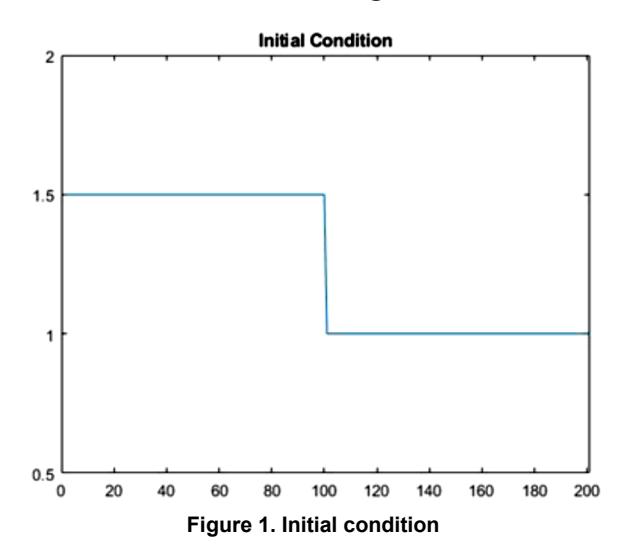
The dam break flow is given by a sudden opening of the gate. The simulation time is set to 10 seconds with 0.5 m distance interval and 0.001 s time interval. Verification can be done with stoker solution because this test case meet the requirements: sudden flow change, flat channel base, and no scouring.
As we can see from Figure 2 the simulation shows a similar flow pattern but quite big oscillation and instability still occur especially in the downstream. Therefore, a numerical filter is needed to handle the shock (Harlan et al., 2019). Correction factor fk = 0.99 is used.
The difference in error between the simulation results without using a filter with the simulation results using a filter is calculated with the Root Mean Square Error (RMSE) method. RMSE is the standard deviation of the residuals (predictions errors). Residuals are a measure of how far the data points to the regression line are. Simulation using numerical filter in Figure 3 shows a smoother and more stable result without oscillation compared to Figure 2. The result from FTCS numerical scheme is compared to the analytical solution by calculating RMSE value at 5 seconds and 10 seconds time steps. The application of numerical filter can decrease RMSE value, so the filter is recommended to be used in the next case.
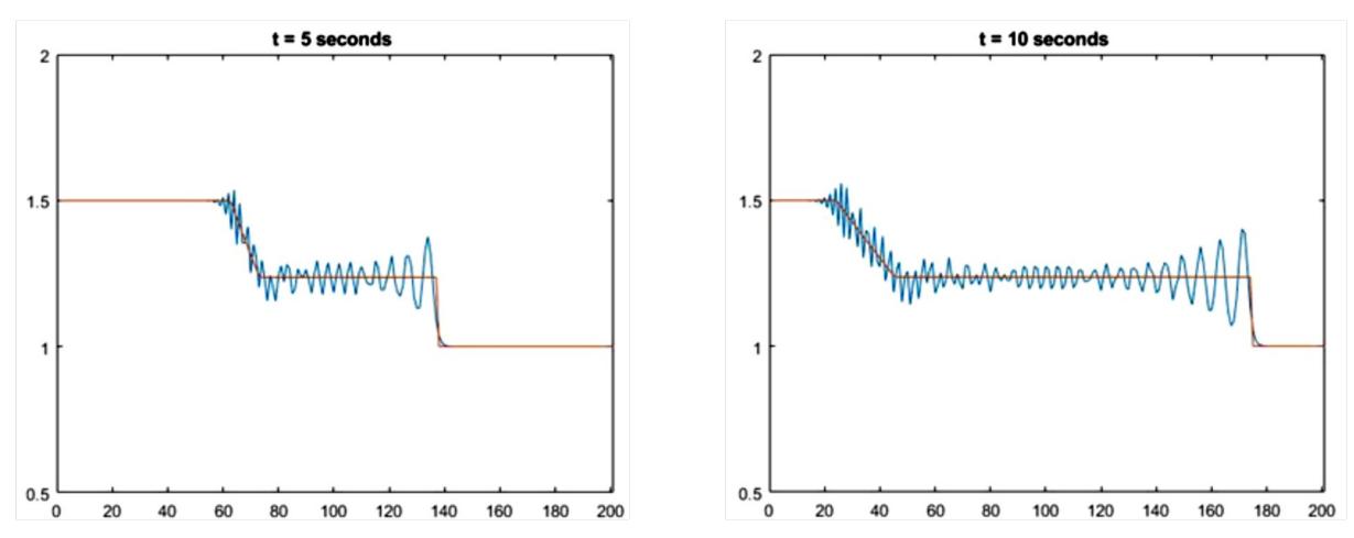
Figure 2. Simulation result at (a) time=5 seconds and (b) time=10 seconds
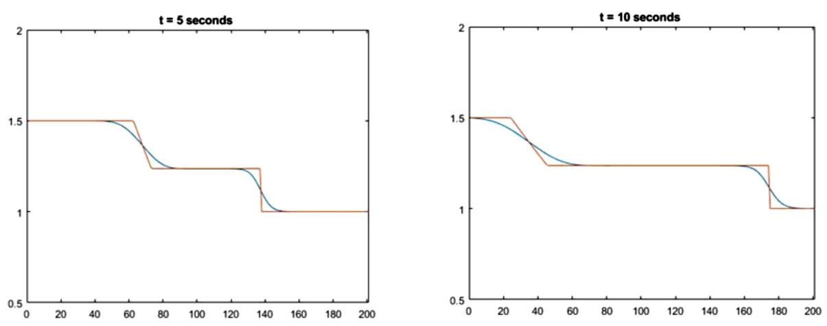
Figure 3. Simulation result at (a) time=5 seconds and (b) time=10 seconds using hansen filter
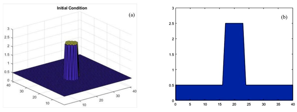
Figure 4. Initial condition of circular dam break from (a) a perspective view and (b) a middle cross-section
Tabel 1. Error summary report
| RMSE | |||
|---|---|---|---|
| t(s) | FTCS without filter | FTCS with filter | Choosen choice |
| 5 | 3.36% | 2.48% | FTCS with Filter |
| 10 | 4.72% | 2.69% | FTCS with Filter |
| cumulative | 4.04% | 2.59% | FTCS with Filter |
3.2 Circular dam break 2d
The second case about a circular dam break is similar to cases presented in refers to (Ginting and Mundani, 2019) and (Delis and Katsaounis, 2005). This case is used to check the reliability of FTCS numerical scheme with numerical filter when it comes to solve a complex shallow flow problem in 2D. the domain is a \(40 \times 40\) m square with no slope nor friction. The initial condition is that two regions of still water are separated by a cylindrical wall with 2.5 m radius as shown in Figure 4.
Water depth inside the cylinder wall is 2.5 m and the outside wall consists of 0.5 m water. The water is assumed to be at rest with no initial velocity and all boundaries are set to wall boundary. The total simulation time is 4.7 seconds with 0.005 s time interval and calculated in a 41 x 41 grid.
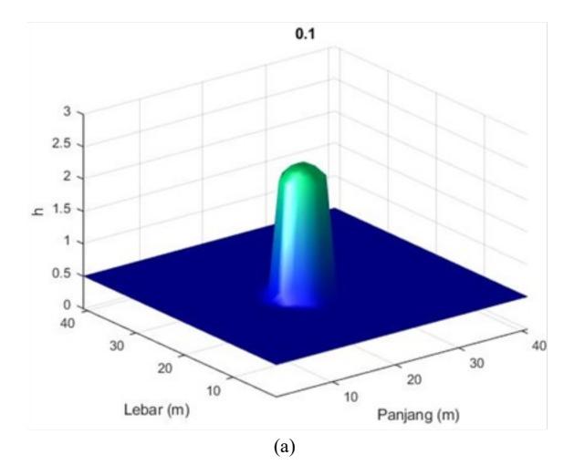
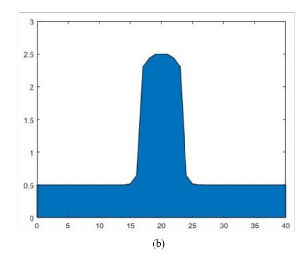
Figure 5. Result of FTCS scheme for circular dam break at 0.1 s from (a) a perspective view and (b) a middle cross-section
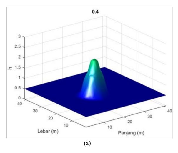
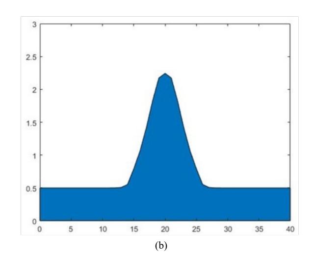
Figure 6. Result of FTCS scheme for Circular Dam Break at 0.4 s from (a) a perspective view and (b) a middle cross-section
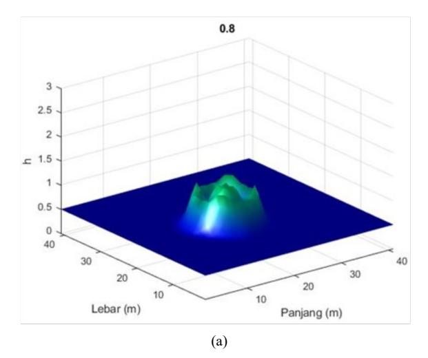
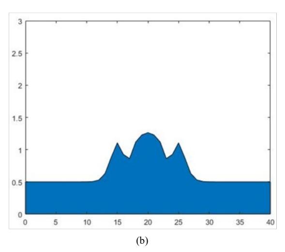
Figure 7. Result of FTCS scheme for circular dam break at 0.8 s from (a) a perspective view and (b) a middle cross-section
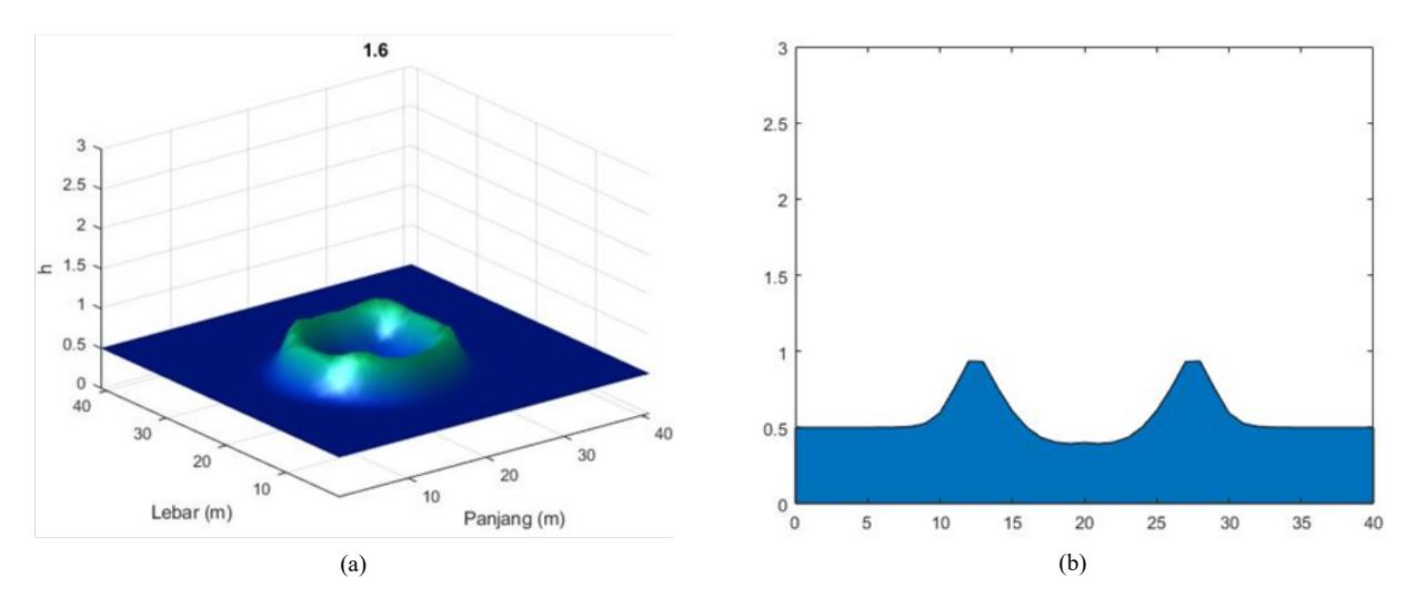
Figure 8. Result of FTCS scheme for circular dam break at 1.6 s from (a) a perspective view and (b) a middle cross-section
Figure 9. Result of FTCS scheme for circular dam break at 3.8 s from (a) a perspective view and (b) a middle cross-section
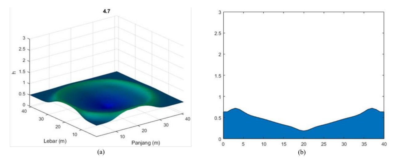
Figure 10. Result of FTCS scheme for circular dam break at 4.7 s from (a) a perspective view and (b) a middle cross-section
The simulation is also conducted without using Hansen's Filter. The model crashes at 2.95 seconds and already shows oscillation or instability from the start. Whereas, all the results from Figure 4 to Figure 10 with Hansen's Filter are stable and smooth. They also show similar results to those presented in refers to (Ginting and Mundani, 2019).
4. Conclusion
- Based on the analysis above, simulation of 1D dambreak using FTCS numerical scheme which is modeled on a 100 m longitudinal channel with initial conditions in the upstream water depth h1 = 1.5 m and downstream h2 = 0.5 m shows a similar flow pattern to analytical solution but it is not stable and quite big oscillation still occurs.
- Hansen Filter can significantly reduce the oscillation due to numerical instability. It can also increases accuracy even though it shows a less accurate wavefront and moveable bed situation. Furthermore, a numerical scheme can be applied to 2D dam-break simulations. In this case, the FTCS numerical scheme was applied to the circular dam break case.
- The initial conditions given in the 2D circular dam break simulation are 2.5 m water depth inside the cylinder wall and the outside wall consists of 0.5 m water. The total simulation time is 4.7 seconds with 0.005 s time interval and calculated in a 41 x 41 grid. Overall, it can be concluded that FTCS numerical scheme with numerical filter can be used to solve shallow flow problem 2D such as circular dam break simulation.
- However, additional investigation and verification are required for further application of this method.
5. Acknowledgment
This study is supported by P3MI LPPM ITB and KK ITB Grant Research 91c/I1.C01/PL/2019.
6. References
- Adityawan, M. B., and Tanaka, H. (2012): Bed stress assessment under solitary wave run-up, Earth, Planets and Space, 64(10), 945–954.
- Brufau, P., and García-Navarro, P. (2003): Unsteady Free Surface Flow Simulation Over Complex Topography with A Multidimensional Upwind Technique, Journal of Computational Physics, 186(2), 503–526.
- Delis, A. I., and Katsaounis, Th. (2005): Numerical solution of the two-dimensional shallow water equations by the application of relaxation methods, Applied Mathematical Modelling, 29 (8), 754–783.
- Delis, A. I., and Skeels, C. P. (1998): TVD schemes for open channel flow, International Journal for Numerical Methods in Fluids, 26(7), 791-809.
- Farid, M., Yakti, B. P., Rizaldi, A., and Adityawan, M. B. (2016): Finite Difference Numerical Scheme for Simulating Dam Break Flow, The 5th HATHI International Seminar on Water Resilience in a Changing World.
- Ginting, B., and Mundani, R.-P. (2019): Comparison of Shallow Water Solvers: Applications for Dam-
- Break and Tsunami Cases with Reordering Strategy for Efficient Vectorization on Modern Hardware, Water, 11(4), 639.
- Harlan, D., Adityawan, M. B., Natakusumah, D. K., and Lely Hardianti Zendrato, N. (2019): Application of Numerical Filter to a Taylor Galerkin Finite Element Model for Movable Bed Dam Break Flows, International Journal of GEOMATE, 16 (57).
- Kawahara, M., and Umetsu, T. (1986): Finite Ement Method for Moving Boundary Problems in River Flow, International Journal for Numerical Methods in Fluids, 6(6), 365–386.
- Lai, W., and Khan, A. A. (2011): Discontinuous Galerkin Method for 1D Shallow Water Flow with Water Surface Slope Limiter, 5(3), 10.
- Welahettige, P., Vaagsaether, K., and Lie, B. (2018): A Solution Method for One-Dimensional Shallow Water Equations Using Flux Limiter Centered Scheme for Open Venturi Channel, The Journal of Computational Multiphase Flows, 10(4), 228–238.
- Yakti, Bagus Pramono., Adityawan, M.B., Farid, Mohammad., Suryadi, Yadi., Nugroho, Joko., Hadihardaja, Iwan Kridasantausa. (2018): Modeling of Flood Propagation due to the Failure of Way Ela Natural Dam, MATEC Web of Conferences 147, 03009.
Development of FTCS Artificial Dissipation...