
2.2 Wave number k, wave constant G and wave amplitude function equations
Hutahaean (2019b) formulated a weighted total acceleration equation for a function f(x, z, t) in the form of, \[\frac{Df}{dt} = \gamma \frac{df}{dt} + u \frac{df}{dx} + \gamma_z w \frac{df}{dz}\]
\(\boldsymbol{u}\) is the velocity of fluid particle in the horizontal- \(\boldsymbol{x}\) direction, \(\boldsymbol{w}\) is the velocity of fluid particle in the vertical- \(\boldsymbol{z}\) direction, \(\boldsymbol{t}\) is time, \(\boldsymbol{\gamma}\) and \(\boldsymbol{\gamma}_z\) is weighting coefficient.
Equation to calculate wave number k or dispersion equation in the form of,
\[\gamma^2 \sigma^2 \left(1 - \frac{kA}{2}\right) + \frac{\gamma^2 \sigma^2}{4} (1 - \gamma_z) kA = gk \left(1 - \frac{kA}{2}\right)^2\] (6)
Where k is the wave number whose values is sought,
\(\sigma = \frac{2\pi}{T}\) is angular frequency, T is wave period, g is gravitational velocity, A is wave amplitude.
Weighting coefficient value for time- t(y) differential
\[\frac{1}{2} - \gamma + \frac{1}{2}\gamma^2 = \frac{\varepsilon}{c^{s_*}}(1 + \gamma) \tag{7}\]
Where for \(\delta t = \frac{2\epsilon}{\sigma}\), \(\epsilon\) is a very small number, \(\gamma = 3\) is obtained for all wave period and for all values of \(\epsilon\). Weighting coefficient value for differential against vertical-z (\(\gamma_z\)) axis.
\[-\frac{\gamma^2}{2}c_1 + \gamma - \frac{c_1}{2} - \frac{1}{2}(-\gamma c_1 - c_1)\] \[-\left(\gamma + 1 + \frac{1}{2}\right)c_2\gamma_z + \frac{c_1}{2}\gamma_z^2 = 0\] (8)
\(c_1=c_2=\cosh(2.415\pi)=\sinh(2.415\pi)\), for \(\gamma=3\), \(\gamma_z=1.630\) is obtained. The constant 2.415 is obtained from the adjustment of breaker depth that was done in Chapter V.
Wave amplitude function equation
\[A = \frac{2Gk}{\sigma v} \cosh(2.415\pi) \left(1 - \frac{kA}{2}\right) \tag{9}\]
In a deep water where wave amplitude A is a known input, the calculation of wave constant G is done with (9).
\[G = \frac{\sigma \gamma A}{2k\cosh(2.415\pi)\left(1 - \frac{kA}{2}\right)}\](10)
2.3 The result of equation in deep water
In the case that convective equation is ignored then (6) becomes,
\[\gamma^2 \sigma^2 = gk \left( 1 - \frac{kA}{2} \right) \tag{11}\]
This equation is a quadratic equation for wave number k, where there is an equation root if the value of determinant D is bigger than or equal to zero. The wave amplitude is maximum in the equation if determinant D = 0, where the following is obtained
\[A_{max} = \frac{g}{2\gamma^2 \sigma^2} \tag{12}\]
\(A_{max}\) in (11) is wave amplitude maximum for a wave period
Deep water depth \(h_0\) is obtained with the following equation
\[h_0 = \frac{1}{k} \left( 2.415\pi - \frac{kA}{2} \right) \tag{13}\]
Table 1 shows the result of the calculation for a number of wave periods T, where \(A_{max}\) is used as the wave amplitude. Wave height H, is calculated with equation \(H = \eta_{max} - \eta_{min}\), where \(\eta_{max}\) is wave crest elevation and \(\eta_{min}\) is wave trough elevation, both of which are obtained from water surface equation (2), using \(\cos \sigma t = 1\).
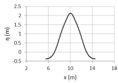
Figure 1. The profile of a wave with wave period 8 sec., in one wave length
Wave-steepness \(\frac{H}{L} = 0.28\), where considering the calculation used maximum wave Amplitude A that was calculated using (12), then wave steepness is critical
Table 1. Characteristic of wave profile in deep water
| T (sec) | H (m) | L (m) | \(\frac{H}{L}\) | \(\frac{H}{A}\) | \(\frac{\eta_{max}}{H}\) |
|---|---|---|---|---|---|
| 6 | 1,409 | 5,026 | 0,28 | 2,865 | 0,851 |
| 7 | 1,918 | 6,842 | 0,28 | 2,865 | 0,851 |
| 8 | 2,506 | 8,936 | 0,28 | 2,865 | 0,851 |
| 9 | 3,171 | 11,309 | 0,28 | 2,865 | 0,851 |
| 10 | 3,915 | 13,962 | 0,28 | 2,865 | 0,851 |
| 11 | 4,737 | 16,894 | 0,28 | 2,865 | 0,851 |
| 12 | 5,638 | 20,105 | 0,28 | 2,865 | 0,851 |
| 13 | 6,617 | 23,595 | 0,28 | 2,865 | 0,851 |
| 14 | 7,674 | 27,365 | 0,28 | 2,865 | 0,851 |
| 15 | 8,81 | 31,413 | 0,28 | 2,865 | 0,851 |
Table 2. Type of wave based on Wilson criteria (1963)
| Wave Type | \(\frac{\eta_{max}}{H}\) |
|---|---|
| Airy waves | < 0.505 |
| Stoke's waves | < 635 |
| Cnoidal waves | \[0.635 < \frac{\eta_{max}}{H} < 1\] |
| Solitary waves | = 1 |
wave steepness. The critical wave steepness is bigger than the criteria of Michell (1893) i.e. \(\frac{H}{L} = 0.142\). The comparison between wave height and wave amplitude is \(\frac{H}{A}\) = 2.865 which is bigger than 2. Therefore, the relation between wave height and wave amplitude is H = 2A cannot be determined. The obtained Wilson parameter is \(\frac{\eta_{max}}{H} = 0.851\). Based on Wilson criteria (1963), Table 2, the value of the parameter shows that the wave profile has a cnoidal wave type, with wave profile presented in Figure 1. for wave period T = 8 sec.
2.4 Comparison with Wiegel equation
Using data from an observation, Wiegel (1949-1964) formulated the relation between wave period T and maximum wave height \(H_{max}\) in a wave period, i.e.
\[T_{Wieg} = 15.6 \sqrt{\frac{H_{max}}{g}} \tag{14}\]
The comparison was done to calculate \(T_{wieg}\) in (14) using wave height from the result of a calculation using a model, and as an input in the model is wave period Tand wave amplitude calculated with (12), so that wave height that was obtained is wave height maximum \(H_{max}\) in the related wave period. The calculation was done using two \(\gamma\) values as presented in Table 3.
Table 3 shows that at \(\gamma = 3\), \(T_{Wieg}\) that was obtained is almost equal to T which is a wave period to calculate \(H_{max}\) with model. Whereas for \(\gamma = 2.97102\), it can be stated that \(|T - T_{Wieg}|\) is equal to zero. From this comparison, a conclusion can be made that the values of Y, Yz and equations formulated in this research
Table 3. The comparison with wiegel equation.
| T (sec) | \[\gamma = 3.0\] \[\gamma_z = 1.63164\] | • | \(\gamma = 2.97102\) \(\gamma_z = 1.60095\) | ||
|---|---|---|---|---|---|
| Hmax (m) | TWieg (sec) | Hmax (m) | TWieg (sec) | ||
| 6 | 1,40943 | 5,91305 | 1,45118 | 6 | |
| 7 | 1,9184 | 6,89858 | 1,97523 | 7,00002 | |
| 8 | 2,50569 | 7,88412 | 2,57992 | 8,00007 | |
| 9 | 3,1713 | 8,86969 | 3,26522 | 9,00007 | |
| 10 | 3,91518 | 9,85522 | 4,03119 | 10,0002 | |
| 11 | 4,73746 | 10,8408 | 4,87774 | 11,0002 | |
| 12 | 5,63796 | 11,8264 | 5,80504 | 12,0003 | |
| 13 | 6,61695 | 12,8121 | 6,81286 | 13,0004 | |
| 14 | 7,67409 | 13,7976 | 7,90155 | 14,0006 | |
| 15 | 8,80954 | 14,7831 | 9,07066 | 15,0006 | |
correspond with the result of Wiegel (1949-1964) research which is the result of an observation.
3. Governing Equations of Shoaling-Breaking Model
3.1 Energy conservation equation
a. Mass conservation of a potential velocity component
Equation 1 was done at a characteristic point, i.e. a point where coskx = sinkx = cosot = sinot. And as function x, coskx is used.
\[\Phi(x,z,t) = 2G \cos kx \cosh k(h+z) \sin \sigma t \tag{15}\]
\[u = -\frac{d\Phi}{dx} = 2Gk \ sinkx \ coshk (h + z)sin \ \sigma t\]\[-2\frac{dG}{dx} \ coskx \ coshk (h + z)sin \ \sigma t \tag{16}\]
\[\frac{du}{dx} = 2Gk^{2} coskx coshk(h + z) sin \sigma t\] \[+2 \frac{dGk}{dx} sinkx coshk(h + z) sin \sigma t\] \[+2k \frac{dG}{dx} sinkx coshk(h + z) sin \sigma t\] \[-2 \frac{d^{2}G}{dx^{2}} coskx coshk(h + z) sin \sigma t \qquad (17)\]
\[w = -\frac{d\Phi}{dz} = -2Gk \; coskx \; sinhk \, (h+z) sin \; \sigma t \qquad (18)\]
\[\frac{dw}{dz} = -2G k^2 coskx sinhk(h + z) sin \sigma t\] (19)
Substitute (16) and (19) to the continuity equation \(\frac{du}{dv} + \frac{dw}{dz} = 0\), and it is done at the characteristic point,
\[G\frac{dk}{dr} + 2\frac{dG}{dr}k - \frac{d^2G}{dr^2} = 0 (20)\]
Considering that in G there is a wave energy, this equation can also be called energy conservation equation. The existence of the term \(\frac{\mathbf{a}^2 \mathbf{c}}{\mathbf{a} \mathbf{x}^2}\) has caused
difficulties in using conservation equation (20). To get rid of the term \(\frac{\mathbf{a}^2 \mathbf{c}}{\mathbf{a} \mathbf{x}^2}\), Hutahaean (2019c) conducted an approximation where (18) is differentiated against horizontal-\(\mathbf{x}\) axis, then the terms \(\frac{\mathbf{a}^3 \mathbf{c}}{\mathbf{a} \mathbf{x}^3}\) and \(\frac{\mathbf{a}^2 \mathbf{k}}{\mathbf{a} \mathbf{x}^2}\) are regarded as very small number that can be ignored, whereas \(\frac{\mathbf{a}^2 \mathbf{c}}{\mathbf{a} \mathbf{x}^2}\) is substituted with (3), and a new conservation equation is obtained, i.e.
\[3\frac{dg}{dx}\frac{dk}{dx} + 2kG\frac{dk}{dx} + 4k^2\frac{dg}{dx} = 0\] (21)
This equation is an approximation equation. To obtain a better equation, a complete velocity potential equation (1) is used at the continuity equation \(\frac{du}{dx} + \frac{dw}{dz} = 0\), and is done in the following section.
b. Mass Conservation of a complete potential velocity
From (1).
\[u = -\frac{d\Phi}{dx} = -Gk\cosh k(h+z)(-\sinh x + \cosh x)\sin \sigma t\] \[-\frac{dGk}{dx}\cosh k(h+z)(-\sinh x + \cosh x)\sin \sigma t\] \[-\frac{dG}{dx}k\cosh k(h+z)(-\sinh x + \cosh x)\sin \sigma t\] \[-\frac{d^2G}{dx^2}\cosh k(h+z)(\cosh x + \sinh x)\sin \sigma t \qquad (22)\]
\[w = -\frac{d\Phi}{dz} = -Gk\sinh k (h+z)(\cosh x + \sinh x)\sin \sigma t\] \[\frac{dw}{dz} = -Gk^2\sinh k (h+z)(\cosh x + \sinh x)\sin \sigma t \qquad (23)\]
(22) and (23), are substituted to continuity equation \(\frac{du}{dx} + \frac{dw}{dz} = 0\) and are done at the characteristic point, and the following is obtained
\[\frac{\mathbf{d}^2 \mathbf{G}}{\mathbf{d} \mathbf{v}^2} = \mathbf{0} \tag{24}\]
Substitute (24) to (18), energy conservation equation as well as mass conservation equation were obtained in other form, i.e.
\[G\frac{dk}{dx} + 2\frac{dG}{dx}k = 0 (25)\]
This is exact equation, not an approximation equation as in (20).
3.2 Wave amplitude function equation
Hutahaean (2019d) shows that wave constant, i.e. wave number k and wave constant G can be obtained by using one velocity potential component where either using the cosine component or sine component, similar wave constants equations will be obtained. By substituting one velocity potential component at the surface kinematic boundary condition and integrating the formed equation against time-t, Hutahaean (2019b) obtained wave amplitude function equation, i.e.
\[A = \frac{2Gk}{\sigma \gamma} \cosh(2.415\pi) \left(1 - \frac{kA}{2}\right) \tag{26}\]
This equation is differentiated against horizontal- x axis
\[\frac{\mathrm{d}A}{\mathrm{d}x} - \frac{2}{\sigma\gamma} \cosh{(2.415\pi)} \left(1 - \frac{\mathrm{k}A}{2}\right) \left(k \, \frac{\mathrm{d}G}{\mathrm{d}x} + G \, \frac{\mathrm{d}k}{\mathrm{d}x}\right) = 0\]
Substitute \[\frac{dG}{dx} = -\frac{G}{2k}\frac{dk}{dx}\] from (22)
\[\frac{dA}{dx} - \frac{2}{\sigma y} \cosh(2.415\pi) \left(1 - \frac{kA}{2}\right) \left(-k \frac{G}{2k} \frac{dk}{dx} + G \frac{dk}{dx}\right) = 0 \qquad (27)\]
3.3 Wave number conservation equation
From the method of variable separation in the completion of Laplace equation, where velocity potential is considered as a multiplication of three functions, i.e \(\Phi(x,z,t) = X(x)Z(z)T(t)\), where X(x) is just a function of x, Z(z) is just a function of z and Z(z) and Z(z) is just a function of time z, where in (1), Z(z) = cosk(h + z), then the following should apply,
\[\frac{dk\left(h+z\right)}{dx} = 0 \tag{28}\]
This equation is a wave number conservation equation. Equation (28) is done at \(z = \eta(x, t)\) and done at the characteristic point, then the wave number equation becomes,
\[\frac{dk\left(h + \frac{A}{2}\right)}{dx} = 0 \tag{29}\]
4. Shoaling-Breaking Equation
A wave moving from deeper water to shallower water will experience a change in its constant, i.e. \(\frac{3G}{ax}\), \(\frac{3k}{ax}\) and \(\frac{3A}{ax}\). To calculate the change in the three constants, three equations are needed. Those equations are energy conservation equation, wave amplitude function equation and wave number conservation equation. The three equations formed linear simultaneous equation with variables \(\frac{3G}{ax}\), \(\frac{3k}{ax}\) and \(\frac{3A}{ax}\) that can be completed using Gauss elimination method or the like. Bearing in mind that the form of the three equations is simple linear equation so that from the three equations, equations for \(\frac{3G}{ax}\), \(\frac{3k}{ax}\) and \(\frac{3A}{ax}\), so that matrix operation is no longer needed to complete it. In the following sections, calculation method will be formulated with the two methods.
4.1 Using matrix operation
As has been stated that the three change equations of the wave constant will form a system of linear equation with variables \(\frac{dG}{dx}\), \(\frac{dk}{dx}\) and \(\frac{dA}{dx}\). The equation can be written in the form of matrix as follows.
\[\begin{bmatrix} a_{11} & a_{12} & a_{13} \\ a_{21} & a_{22} & a_{23} \\ a_{31} & a_{32} & a_{33} \end{bmatrix} \begin{pmatrix} x_1 \\ x_2 \\ x_3 \end{pmatrix} = \begin{pmatrix} b_1 \\ b_2 \\ b_3 \end{pmatrix}\](30)
Where \[x_1 = \frac{dG}{dx}\]; \(x_2 = \frac{dk}{dx}\); \(x_3 = \frac{dA}{dx}\)
\[G_{x+\delta x} = G_x + \delta x \frac{dA}{dx} \tag{31}\]
\[k_{x+\delta x} = k_x + \delta x \frac{dk}{dx} \tag{32}\]
\[A_{x+\delta x} = A_x + \delta x \frac{dA}{dx} \tag{33}\]
Next is a discussion on matrix coefficients in (30)
a. Energy equation
Energy conservation equation (23), is written as
\[2k\frac{dG}{dx} + G\frac{dk}{dx} = 0 \tag{34}\]
Matrix coefficients of this equation are.
\[a_{11} = 2k\]; \(a_{12} = G\); \(a_{13} = 0\); \(b_1 = 0\)
b. Wave amplitude function equation
From (24) i.e.
\[\frac{dA}{dx} - \frac{2}{\sigma \gamma} \cosh(2.4\pi) \left(1 - \frac{kA}{2}\right) \left(k \frac{dG}{dx} + G \frac{dk}{dx}\right) = 0\] (35)
Matrix coefficients of this equation are.
\[a_{21} = -\frac{2}{\sigma\gamma} cosh(2.415\pi) \left(1 - \frac{kA}{2}\right) k\]
\[a_{22} = -\frac{2}{\sigma \gamma} \cosh(2.415\pi) \left(1 - \frac{kA}{2}\right) G\]
\[a_{23} = 1 \cdot b_2 = 0\]
c. Wave number conservation equation
Wave number conservation equation (36) is,
\[\frac{dk\left(h + \frac{\bar{A}}{2}\right)}{dx} = 0 \tag{36}\]
Matrix coefficients in this equation are
\[a_{31} = 0\]; \(a_{32} = \left(h + \frac{A}{2}\right)\); \(a_{33} = \frac{k}{2}\); \(b_3 = -k \frac{dh}{dx}\)
4.2 Simple equation
From the linear equation, simple equation can be formed, so that in the calculation the completion of simultaneous linear equations operation is not needed.
\(\frac{\mathbf{a}\mathbf{G}}{\mathbf{a}\mathbf{x}}\) in (35) is substituted with energy conservation
\[\frac{dA}{dx} = \frac{G}{\sigma y} \cosh(2.415\pi) \left(1 - \frac{kA}{2}\right) \frac{dk}{dx}\] (37)
This equation is substituted to wave number conservation
\[\left(h + \frac{A}{2}\right)\frac{dk}{dx} + k\frac{dh}{dx} + \frac{Gk}{2\sigma\gamma}cosh(2.415\pi)\left(1 - \frac{kA}{2}\right)\frac{dk}{dx} = 0\] (38)
The calculation step is to calculate \(\frac{dk}{dt}\) with (38), then is calculated with (37). Next, Taylor series is done to obtain new wave number and wave amplitude values.
\[k_{x+\delta x} = k_x + \delta x \frac{\mathrm{d}k}{\mathrm{d}x}\]
\[A_{x+\delta x} = A_x + \delta x \frac{\mathrm{d}A}{\mathrm{d}x}\]
The calculation of \(\frac{a_G}{a_X}\) was done analytically. The energy conservation equation (24) can be written as,
\[\frac{1}{G}\frac{dG}{dx} = -\frac{1}{2k}\frac{dk}{dx} \tag{39}\]
Both terms of the equation are multiplied with dx and then are integrated against horizontal-x axis.
\[\int_{r}^{x+\delta x} \frac{\mathrm{d}G}{G} = -\frac{1}{2} \int_{r}^{x+\delta x} \frac{\mathrm{d}k}{k}\]
The following is obtained
\[G_{x+\delta x} = e^{\left(\ln G_x - \frac{1}{2}(\ln k_{x+\delta x} - \ln k_x)\right)}\] (40)
5. The Result of Shoaling-Breaking Model
5.1 Breaker height comparator
The result of breaker height model was calibrated against the average value of 5 (five) breaker height indexes. The breaker height index equations used as comparators are breaker height index (BHI) equations from Komar and Gaughan (1972), Larson, M. and Kraus, N.C. (1989), Smith and Kraus (1990), Gourlay (1992) and Rattana Pitikon and Shibayama (2000). Breaker depth is adjusted with the result of breaker depth from SPM (1984).
Komar and Gaughan (1972)
\[\frac{H_b}{H_0} = 0.56 \left(\frac{H_0}{L_0}\right)^{-\frac{1}{5}} \tag{41}\]
Larson and Kraus (1989),
\[\frac{H_b}{H_0} = 0.53 \left(\frac{H_0}{L_0}\right)^{-0.24} \tag{42}\]
Smith and Kraus (1990),
\[\frac{H_b}{H_0} = (0.34 + 2.74m) \left(\frac{H_0}{L_0}\right)^{-0.30 + 0.88m}\] (43)
Gourlay (1992),
\[\frac{H_b}{H_0} = 0.478 \left(\frac{H_0}{L_0}\right)^{-0.28}\]
(44)
Rattana Pitikon and Shibayama (2000):
\[\frac{H_b}{H_0} = (10.02m^3 - 7.46m^2 + 1.32m + 0.55) \left(\frac{H_0}{L_0}\right)^{-\frac{1}{5}}\] (45)
\(H_0\) is deep water wave height, \(L_0\) is deep water wave length (calculated using linear wave theory,
\[k_0 = \frac{\sigma^2}{g}\], \(L_0 = \frac{2\pi}{k_0}\)), \(m\) is bottom slope and \(H_b\) is breaker height.
5.2 Breaker depth comparator
As a comparator of the result of breaker depth calculation, breaker depth index from SPM (1984) is used, with breaker height as input that is obtained from
\[\frac{h_b}{H_b} = \frac{1}{b - \left(\frac{aH_b}{gT^2}\right)} \quad \text{atau} \quad h_b = \frac{H_b}{b - \left(\frac{aH_b}{gT^2}\right)}\] \[a = 43.75(1 - e^{-19.0m}) \quad b = \frac{1.56}{1 + e^{-19.5m}}\] \[h_b \quad \text{breaker depth.}\] (46)
5.3 Breaker height calculation
The breaker height \(H_{br}\) calculation was done using water wave surface equation (2)., where \(\cos \sigma t = 1\) was used. As an input for the equation is wave parameter at breaker point, i.e. wave-number \(k_{br}\), breaker depth \(h_{br}\) and breaker wave amplitude \(A_{br}\). Considering that there are summation of two waves in (2) or (4), then breaker wave amplitude should be divided with 2, or \(A = \frac{A_{br}}{2}\) was used. The next input berikutnya is the value of wave constant G at breaker point. The adjustment with breaker height from breaker heigh index (BHI) equation, was done by multiplying wave constant G at breaker point with a coefficient \(c_G\).
The adjustment of breaker depth with the result of SPM (1984) was done by changing deep water constant. The definition of deep water depth is \(\tanh k \left(h_0 + \frac{A_0}{2}\right) = 1\) atau \(k \left(h_0 + \frac{A_0}{2}\right) = \alpha \pi\). The deep water constant is \(\alpha \pi\). Using the value of \(\alpha = 2.415\), breaker depth \(h_b\) that corresponds to the breakerdepth from SPM (1984) was obtained.
a. Breaker height model without adjustment, \(c_G = 1\)
Table 3 shows the result of breaker height calculation without correcting the value of G, or \(c_G = 1\). The value of breaker height model is bigger than the value of breaker height from the average value of Breaker Height Index (BHI), but it can be stated that the difference is relatively small. Table 4 presents the comparison between breaker height model and breaker minimum and breaker height maximum of the five Breaker Height Index Equations and it is found that breaker height model is bigger than breaker height maximum, but with relatively small difference, with differences between 0.03 m-0.15 m.
b. Breaker height model with adjustment, \(c_a = 0.878\)
Furthermore, Table 6 shows the result of the calculation using coefficient correction \(c_G = 0.878\), and the breaker height that is equal to the value of breaker height average from BHI equation. From the result of the comparison, it can stated that water wave equations that were developed in this research including weighted total acceleration equation with its weighting coefficient, i.e. \(\gamma\) and \(\gamma_z\) provides the result of breaker height that corresponds to the result of physical model.
The wave profile at breaker point for wave period T = 8 sec is presented in Figure 2., where the calculation uses \(c_G = 0.878\). It shows that in general, the form of the wave profile is cnoidal wave.
Table 4. The result of breaker height calculation without correction \((c_G = 1)\).
| T (sec) | H0 (m) | Hbr Model (m) | Hbr (BHI) (m) | hb (Model) (m) | hb (SPM) (m) |
|---|---|---|---|---|---|
| 6 | 1,409 | 1,838 | 1,615 | 2,019 | 2,019 |
| 7 | 1,918 | 2,502 | 2,198 | 2,749 | 2,748 |
| 8 | 2,506 | 3,269 | 2,871 | 3,59 | 3,59 |
| 9 | 3,171 | 4,137 | 3,634 | 4,543 | 4,543 |
| 10 | 3,915 | 5,106 | 4,486 | 5,612 | 5,609 |
| 11 | 4,737 | 6,179 | 5,428 | 6,789 | 6,787 |
| 12 | 5,638 | 7,353 | 6,46 | 8,079 | 8,077 |
| 13 | 6,617 | 8,629 | 7,582 | 9,483 | 9,479 |
| 14 | 7,674 | 10,008 | 8,793 | 10,998 | 10,993 |
| 15 | 8,81 | 11,49 | 10,094 | 12,624 | 12,62 |
Note: Ho: deep water wave height
Table 5. The Comparison of breaker height model (C<sub>G</sub> =1), with breaker height maximum and minimum
| T (sec) | H0 (m) | Hbr-min (m) | Hbr-model | Hbr-max (m) |
|---|---|---|---|---|
| 6 | 1,409 | 1,482 | 1,839 | 1,809 |
| 7 | 1,918 | 2,017 | 2,502 | 2,463 |
| 8 | 2,506 | 2,635 | 3,268 | 3,216 |
| 9 | 3,171 | 3,335 | 4,136 | 4,071 |
| 10 | 3,915 | 4,117 | 5,106 | 5,026 |
| 11 | 4,737 | 4,981 | 6,179 | 6,081 |
| 12 | 5,638 | 5,928 | 7,353 | 7,237 |
| 13 | 6,617 | 6,958 | 8,63 | 8,494 |
| 14 | 7,674 | 8,069 | 10,009 | 9,851 |
| 15 | 8,81 | 9,263 | 11,49 | 11,308 |
Table 6. The result of the breaker height calculation using correction coefficienc \(_{\it G}=0.878\)
| T (sec) | H0 (m) | Hbr Model (m) | Hbr (BHI) (m) | hb (Model) (m) | hb (SPM) (m) |
|---|---|---|---|---|---|
| 6 | 1,409 | 1,614 | 1,615 | 2,019 | 2,019 |
| 7 | 1,918 | 2,197 | 2,198 | 2,749 | 2,748 |
| 8 | 2,506 | 2,87 | 2,871 | 3,59 | 3,59 |
| 9 | 3,171 | 3,632 | 3,634 | 4,543 | 4,543 |
| 10 | 3,915 | 4,483 | 4,486 | 5,612 | 5,609 |
| 11 | 4,737 | 5,425 | 5,428 | 6,789 | 6,787 |
| 12 | 5,638 | 6,456 | 6,46 | 8,079 | 8,077 |
| 13 | 6,617 | 7,577 | 7,582 | 9,483 | 9,479 |
| 14 | 7,674 | 8,787 | 8,793 | 10,998 | 10,993 |
| 15 | 8,81 | 10,088 | 10,094 | 12,624 | 12,62 |
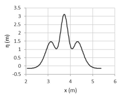
Figure 2. The wave profile at breaker point.
6. Conclusion
- At the breaker point, the model produce breaker height that close to the average breaker height of the five breaker height index equations from the previous researches, and so does the breaker depth produced by the model corresponds to the previous research.
- In general, it can be concluded that the model can estimate breaker height and breaker depth, and maximum wave height in a wave period in deep water. The model is simple in form, and easy to be used, no sophisticated numerical method needed, only with first-order Taylor series. However, a further research needs to be done to other phenomenon contained in a water wave.
- It can be stated that the model development is close to exact without disregarding the non-linear terms at the governing equations that are used. Likewise, at the velocity potential equation a complete solution is used so that the mass conservation equation is well maintained. In the formulation of water surface elevation equation, second order horisontal derivative of water surface equation is neglected. Therefore, the follow up of this model development is the formulation of water surface elevation equation without neglecting the second order derivative.
- The conformity of breaker height model with breaker height from breaker height index indicates that the shoaling that is produced is also good enough, so that it can be used to predict wave height at the coastal water. The application of wave height at the coastal water is among other for design the coastal structure, either the structure strength against wave force and its elevation. The next application is on the development of refraction-diffraction wave model with bathymetry where the shoaling-breaking model at the model of the result of this research can develop a refractiondiffraction model by bathymetry where breaking takes place automatically.
7. References
- Dean, R.G., Dalrymple, R.A. (1991). Water wave mechanics for engineers and scientists. Advance Series on Ocean Engineering.2. Singapore: World Scientific. ISBN 978-981-02-0420-4. OCLC 22907242.
- Gourlay, M.R. (1992). Wave set-up, wave run-up and beach water table: Interaction between surf zone hydraulics and ground water hydarulics. Coastal Eng. 17, pp. 93-144.
- Hutahaean, S. (2019a). Application of Weighted Total Acceleration Equation on Wavelength Calculation. International Journal of Advance Engineering Research and Science (IJAERS). Vol -6, Issue-2, Feb-2019. ISSN-2349-6495(P)/2456-1908(O). https://dx.doi.org/10.22161/ijaers.6.2.31
- Hutahaean , S. (2019b). Modified Momentum Euler Equatuin for Water Wave Modeling. International Journal of Advance Engineering Research and
- Science (IJAERS). Vol-6, Issue-10, Oct-2019. ISSN-2349-6495(P)/2456-1908(O). https:// dx.doi.org/10.22161/ijaers.610.21
- Hutahaean, S. (2019c). Water Wave Modeling Using Wave Constatnt G. International Journal of Advance Engineering Research and Science (IJAERS). Vol-6, Issue-5, May-2019. ISSN-2349-6495(P)/2456-1908(O). https:// dx.doi.org/10.22161/ijaers.6.5.61
- Hutahaean , S. (2019d). Water Wave Modeling Using Complete Solution of Laplace Equation. International Journal of Advance Engineering Research and Science (IJAERS). Vol-6, Issue-8, Aug-2019. ISSN-2349-6495(P)/2456-1908(O). https://dx.doi.org/10.22161/ijaers.6.8.33
- Komar, P.D. and Gaughan, M.K. (1972): Airy wave theory and breaker height prediction. Proc. 13rd Coastal Eng. Conf., ASCE, pp 405-418.
- Larson, M. And Kraus, N.C. (1989): SBEACH. Numerical model for simulating storm-induced beach change, Report 1, Tech. Report CERC 89-9, Waterways Experiment Station U.S. Army Corps of Engineers,
- Rattanapitikon, W. And Shibayama, T.(2000). Vervication and modification of breaker height formulas, Coastal Eng. Journal, JSCE, 42(4), pp. 389-406.
- Smith, J.M. and Kraus, N.C. (1990). Laboratory study on macro-features of wave breaking over bars and artificial reefs, Technical Report CERC-90-12, WES, U.S. Army Corps of Engineers, 232 p.
- Wilson, B.W., (1963). Condition of Existence for Types of Tsunami waves, paper presented at XIII th General
- Wiegel, R.L. (1949). An Analysisis of Data from Wave Recorders on the Pacific Coast of tht United States, Trans.Am. Geophys. Union, Vol.30, pp.700-704.
- Wiegel, R.L. (1964). Oceanographical Engineering, Prentice-Hall, Englewoods Cliffs, N.J.
Study on The Breaker Height...