
2. Methodology
The study began with selecting some earthquake events. The number of the events is not restricted to any values, but statistical significance would be achieved for about thirty events or more. In Section 3 the ground motions were presented and discussed. For each earthquake event, some parameters based on three-component motions were evaluated. The parameters included the peak ground acceleration, velocity, displacement, etc. The number of parameters was immaterial, but parameters commonly adopted by other investigators were investigated herein. These parameters were quantified in Section 4 and there are about nineteen. The correlation coefficients among the parameters were computed considering all earthquake events, and the parameters were grouped based on these coefficients. Three parameters were fully correlated, leaving the remaining sixteen for further analyses. For illustration, at one second period, the spectral acceleration, \(S_a(T=1)\), together with spectral velocity, \(S_{\nu}(T=1)\), the spectral energy input, \(E_{in}(T=1)\), and input power, \(P_{in}(T=1)\), were in one group because any pair were correlated very strong (above 80 percent). In the group, one parameter was selected as the lead parameter, in this case, \(S_a(T=1)\)was the lead parameter of the first group, because it showed the highest correlation, and was widely used in other studies. Other groups were investigated similarly with their own lead parameters. The groups are disjoint sets, and their members vary from one to four parameters. In total there were ten groups to represent all sixteen parameters with high correlation coefficients (above 80 percent). Out of sixteen parameters, however, the first three groups with the spectral acceleration (Sa (T=1)), significant duration \((D_{05-95})\) and peak ground velocity (PGV) as the lead parameters already
represented ten parameters (four for \(S_a(T=1)\), and each three for the other two) with high correlations (above 80 percent). Next, a diagonal matrix consisting of the lead parameters was constructed. The strength of the matrix was measured by its norm, which was used as the basis to define a composite-intensity index. The procedures were repeated for twenty-four periods so that a composite-intensity index spectrum could be created. The index was related to the Mercalli macroseismic intensity scales (MMI) to assign its damage potentials. Consequently, specific damage measures (e.g., drift, plastic collapse mechanism, hysteretic energy dissipation) were not required in this study.
The detailed procedure is described in the following steps.
- 1. Earthquake event collection: The earthquake data were compiled from public domain databases. The data should include events with varying Mercalli macroseismic intensity (MMI). For this purpose, events with intensities higher than VII MMI were considered. The number was so that statistical significance could be represented. A number more than thirty should suffice. They should be statistically independent.
- 2. Seismic parameters: Parameters computed based on three-component motions to characterize a seismic event should be defined, e.g., peak ground acceleration (PGA), velocity (PGV), displacement (PGD), pseudo-spectral acceleration, velocity, displacement (\(S_{pa}(T)\), \(S_{pv}(T)\), \(S_{d}(T)\)), etc. They could be as many as practicable. In this study about nineteen parameters were investigated.
- 3. Correlation coefficients: All seismic parameters were assumed lognormally distributed; hence, their common logarithm values were considered. Correlation coefficients among the lognormally seismic parameters covering all earthquake events were computed and identified. To avoid duplication, parameters with correlation coefficients of unity were screened out from further analyses.
- 4. Parameter grouping: Parameters were grouped based on their correlations. Each group was populated by parameters with correlations higher than 80% among them. The first group was the most populated; the last was the least. The groups were disjoint, when there were ties, the less populated group gave up its tied parameters.
- 5. Lead parameters: For each group, the lead parameter was selected based on the highest correlation in the group, or the most used in other studies.
- 6. Normalization of parameters: The seismic parameters have different units and values, so it is necessary to make them unitless and normalized to make them less likely to produce biases. The normalization process makes each parameter have a unit standard deviation, a mean value of κ and becomes an index. The value of κ is so chosen that no parameter has negative values for all earthquake events after normalization. This process does not alter the correlations among parameters.
- 7. Weight factors of the lead parameters: The total number of the groups was such that the total number of parameters was all covered. As illustration, at period of T=1 second, group 1 was populated by parameters 1,2,3 and 4 or g<sub>1</sub> \((\mathbf{p}_1, \mathbf{p}_2, \mathbf{p}_3, \mathbf{p}_4)\); similarly \(g_2(\mathbf{p}_5, \mathbf{p}_6, \mathbf{p}_7)\), \(g_3(\mathbf{p}_8, \mathbf{p}_9, \mathbf{p}_{10})\), \(g_4\)\((p_{11}), g_5(p_{12}), g_6(p_{13}), g_7(p_{14}), g_8(0), g_9(p_{15}), g_{10}(p_{16}),\)for all sixteen parameters. The bolts are the lead parameters in groups with more than one population. In this case, all sixteen parameters could be represented by ten groups with parameters' correlations higher than 80% in each group. The weight factor of parameter \(p_1\) is \(w_1=4/16\), \(w_2=3/16\) for \(p_5\), \(w_8=0\), and so on. However, it is possible to consider only the three first groups namely \(g_1(\mathbf{p_1},p_2,p_3,p_4),~g_2(\mathbf{p_5},p_6,p_7)\) and \(g_3(\mathbf{p_8}, \mathbf{p_9}, \mathbf{p_{10}})\) covering only ten parameters out of sixteen, with confidence level of about 80% x 10/16 = 50%. Then the weight factors became \(w_1=4/10\), \(w_2=w_3=3/10\) for \(p_1\), \(p_5\), \(p_8\), respectively. Each weighted lead parameter has a mean value of κ multiplied by its respective weight factor, and a unit standard deviation. This process does not alter the correlations among the parameters.
- 8. Composite matrix: A diagonal matrix of the normalized lead parameters as diagonal components was created. Other matrices, a matrix of correlation coefficients among the lead parameters and a diagonal matrix of the weight factors of the lead parameters were also constructed. The composite matrix is the product of these three matrices.
- 9. Composite-intensity index: The intensity of the earthquake event is measured by the strength of the composite matrix indicated by its norm. Any norm can be used and the simplest one, i.e., the Frobenius norm, was adopted in this study. This norm is referred to as the composite-intensity index in this study.
- 10. Damage state: As observed in Step 2, some seismic parameters are period-dependents. Hence the composite-intensity index in Step 9 is also period-dependent, and for an event there is a maximum composite-intensity index at a specific period as well as the associated MMI scale. The maximum composite-intensity indices for all events were then related to their respective MMI scales to produce
Table 1. The earthquake events, peak ground accelerations, peak ground velocities, and their origin.
| NI. | Fauth available availab | Otatia | PGA (g) | F | GV (cm/s | ) | CTATE | ||
|---|---|---|---|---|---|---|---|---|---|
| No | Earthquake event | Station | 1 | 2 | UD | 1 | 2 | UD | - STATE |
| 1 | Tabas, 1978 | Tabas | 0.98 | 0.90 | 0.75 | 104 | 115 | 37 | Iran |
| 2 | Erzinican, 1992 | Erzinican | 0.46 | 0.45 | 0.24 | 68 | 130 | 33 | Turkey |
| 3 | Landers, 1992 | Lucerene | 0.80 | 0.71 | 0.86 | 35 | 94 | 47 | USA |
| 4 | Northridge, 1994 | Rinaldi | 0.90 | 0.41 | 0.86 | 180 | 82 | 48 | USA |
| 5 | Kobe, 1995 | Takatori | 0.80 | 0.43 | 0.16 | 189 | 75 | 22 | Japan |
| 6 | Mexico, 2010 | Michoacan | 0.54 | 0.41 | 0.80 | 63 | 51 | 17 | Mexico |
| 7 | Imperial Valley 7, 1979 | El Centro 6 | 0.28 | 0.16 | 0.08 | 27 | 14 | 2 | USA |
| 8 | Imperial Valley 6, 1979 | Calexico | 0.28 | 0.20 | 0.19 | 18 | 16 | 6 | USA |
| 9 | Kobe, 1995 | Amagasaki | 0.33 | 0.29 | 0.34 | 49 | 39 | 28 | Japan |
| 10 | Mammoth Lakes, 1980 | Mammoth Lakes | 0.44 | 0.39 | 0.26 | 26 | 26 | 10 | USA |
| 11 | N Palm Spring, 1986 | N Palm Springs 529 | 0.71 | 0.67 | 0.38 | 72 | 34 | 13 | USA |
| 12 | Parkfield, 1966 | Temblor | 0.36 | 0.27 | 0.14 | 23 | 15 | 6 | USA |
| 13 | Big Bear, 1992 | Civic Center | 0.55 | 0.48 | 0.20 | 37 | 29 | 13 | USA |
| 14 | Hawai, 2006 | Waimea | 1.09 | 0.68 | 0.75 | 38 | 28 | 19 | USA |
| 15 | L'Aquila, 2009 | V. Aterno | 0.68 | 0.57 | 0.51 | 41 | 43 | 15 | Italy |
| 16 | New Zealand, 2010 | Greendale | 0.77 | 0.72 | 1.26 | 112 | 117 | 35 | New Zealand |
| 17 | San Simeon, 2003 | Templeton Hsptl | 0.48 | 0.44 | 0.27 | 29 | 33 | 18 | USA |
| 18 | Anchorage Alaska, 2018 | St Fish & Game | 0.48 | 0.19 | 0.17 | 36 | 19 | 9 | USA |
| 19 | South Napa, 2014 | Crockett #1 | 0.99 | 0.54 | 0.37 | 22 | 11 | 8 | USA |
| 20 | Managua, 1972 | Managua ESSO | 0.37 | 0.33 | 0.31 | 33 | 33 | 19 | Nicaragua |
| 21 | Chile, 2010 | Angol | 0.93 | 0.68 | 0.28 | 31 | 44 | 22 | Chile |
| 22 | Cape Mendocino, 1992 | Ferndale | 0.38 | 0.27 | 0.07 | 97 | 47 | 7 | USA |
| 23 | Loma Prieta, 1989 | Capitola | 0.51 | 0.44 | 0.56 | 42 | 28 | 17 | USA |
| 24 | Calexico, 2010 | Meloland Rd. | 0.28 | 0.20 | 0.24 | 41 | 34 | 10 | USA |
| 25 | Ferndale, 2010 | Eureka & Dolbeer | 0.33 | 0.23 | 0.08 | 32 | 17 | 5 | USA |
| 26 | Imperial Valley, 1940* | El Centro Array 6 | 0.19 | 0.14 | 0.10 | 66 | 30 | 32 | USA |
| 27 | Morgan Hill, 1984* | Gilroy | 0.66 | 0.39 | 0.34 | 29 | 32 | 17 | USA |
| 28 | N Palm Spring, 1986* | DHSP 517 | 0.59 | 0.57 | 0.28 | 40 | 63 | 25 | USA |
| 29 | Chile Llolleo, 1985* | Llolleo | 0.70 | 0.67 | 0.19 | 48 | 37 | 13 | Chile |
| 30 | Chile Vina Del Mar, 1985* | Vina Del Mar | 0.54 | 0.39 | 0.17 | 61 | 34 | 20 | Chile |
| 31 | Mexico, 1995* | Mexico City | 0.17 | 0.10 | 0.09 | 59 | 38 | 29 | Mexico |
* Two-horizontal component only. The vertical component was constructed as two thirds of the average of the horizontal components.
regression constants. The constants express the relation between the maximum composite-intensity index and the damaging power of the event. (Note: The MMI scales define its scales to the extent of damage of buildings subjected to an earthquake event.) Because the composite-intensity index is period-dependent then the damage state at any period can be accordingly computed; so is the MMI scales based on the regression constants.
These steps were elucidated in the following sections and started with the ground motions analyses considered in the study.
3. Ground Motion Records
For the investigation in this study, a total of thirty-one earthquake ground motions collected worldwide, mostly from the United States, were compiled. The number was immaterial, and the data set was by no means exhaustive, but the statistical significance was expected to be satisfied. They consisted of twenty-five three-component and six two-component strong earthquake records. For the latter, the vertical component was constructed as twothirds of the average of the two horizontal components. They are all the strong earthquakes in character with the modified Mercalli intensity scales of VII-X and were listed in Table 1. To verify the statistical independence of the data, the cross-correlation coefficients were computed for all ninety-three components. The maximum correlation was 0.67 given by the Mexico 1995 earthquake between horizontal-1 and -2 components; all other values were less than this.
4. Earthquake Parameters And Their Correlation Coefficients
The dynamical equation of motion of a mass in threeorthogonal coordinate system is
\[\mathbf{M} \ddot{\mathbf{u}}(t) + \mathbf{C} \dot{\mathbf{u}}(t) + \mathbf{K} \mathbf{u}(t) = -\mathbf{M} \ddot{\mathbf{u}}_{s}(t) \tag{1}\] where M, C, and K are 3 x 3 diagonal matrices of mass, damping, and stiffness, respectively; and ü, ů, and u are the acceleration, velocity, and displacement vectors of the mass. For isotropic system, Eq. (1) reduces to,
\[\ddot{\mathbf{u}}(t) + 2\zeta \omega_n \dot{\mathbf{u}}(t) + \omega_n^2 \mathbf{u}(t) = -\ddot{\mathbf{u}}_g(t) \tag{2}\] where \(\ddot{\mathbf{u}}g = \ddot{\mathbf{u}}g1\), \(\ddot{\mathbf{u}}g2\), \(\ddot{\mathbf{u}}g3\) is the three-component translational ground acceleration vector, \(\zeta\) is the damping, and \(\omega_n\) is the system's natural frequency. The Duhamel integral solution of Eq. (2) for displacement vector is,
\[\mathbf{u}\left(t,\omega_{n},\zeta\right) = -\frac{1}{\omega_{D}} \int_{0}^{t} \ddot{\mathbf{u}}_{g}\left(\tau\right) e^{-\zeta \,\omega_{n}\left(t-\tau\right)} \sin \omega_{D}\left(t-\tau\right) d\tau \qquad (3)\]
Where
\[\omega_D = \omega_n \sqrt{1 - \zeta^2}\]
The following earthquake parameters of a total of nineteen which were mostly developed based on Eq. (3) were investigated. The displacement spectrum is,
\[S_d(\omega_n, \zeta) = \max |\mathbf{u}| (\omega_n, \zeta, t)|\] (4)
Where \(|\mathbf{u}| = \sqrt{\mathbf{u} \cdot \mathbf{u}}\). Similarly, velocity and acceleration spectra are defined as,
\[S_{\nu}(\omega_{n},\zeta) = \max |\dot{\mathbf{u}}(\omega_{n},\zeta,t)| \tag{5}\]
\[S_a(\omega_n, \zeta) = \max |\ddot{\mathbf{u}}(\omega_n, \zeta, t) + \ddot{\mathbf{u}}_g(t)| \tag{6}\]
Peak ground displacement, velocity, and acceleration are defined by,
\[PGD = \max \left| \mathbf{u}_{g}(t) \right| = \lim_{n \to 0} S_{d}(\omega_{n}, \zeta)\] (7)
\[PGV = \max \left| \dot{\mathbf{u}}_{g}(t) \right| = \lim_{\omega \to 0} S_{v}(\omega_{n}, \zeta)\] (8)
\[PGA = \max \left| \ddot{\mathbf{u}}_{g}(t) \right| = \lim_{m \to \infty} S_{a}(\omega_{n}, \zeta) = gA_{0}\] (9)
where g is the gravitational acceleration and \(A_0\) is the peak ground acceleration coefficient.
The Housner spectrum intensity, \(SI(\zeta)\) (Housner, 1952), and seismic energy density, \(SED(\zeta)\), which is the average of the absorbed energy per unit mass, are defined as,
\[SI(\zeta) = \int_{0.1}^{2.5} S_{pv}(T,\zeta) dT\] (10)
\[SED(\zeta) = \int_{T_1}^{T_2} \frac{S_{pv}^2(T,\zeta)}{|T_2 - T_1|} dT\] (11)
where \(S_{pv}(\omega_n,\zeta) = \omega_n S_d(\omega_n,\zeta)\) is the pseudo-velocity spectrum; and the damping is taken to be \(\zeta=5\%\), \(T_1=0.1\), \(T_2=2.5\) seconds.
The Arias intensity (Arias, 1970) is defined as,
\[I_A = \frac{\pi}{2g} \int_0^{t_d} \left| \mathbf{\ddot{u}}_g(t) \right|^2 dt \tag{12}\] where \(t_d\) is the end-time of the record.
Campbell and Bozorgnia (2012) investigated the cumulative absolute velocity (CAV) extensively. They related CAV to the macroseismic intensities \(I_{MM}\) (US), \(I_{JMA}\) (Japan), and \(I_{EMS}\) (Europe). They suggested that CAV was the most stable IM to correlate with damage potentials. There were some others who also studied this CAV or its variants (e.g., Kramer and Mitchell, 2006). A slightly different version, denoted herein as \(CAV_{MM}\), is investigated, and defined as,
\[CAV_{MM} = g \int_{0}^{t_d} H\left(\frac{\left|\mathbf{\ddot{u}}_g(t)\right|}{g} - 0.025\right) \frac{\left|\mathbf{\ddot{u}}_g(t)\right|}{g} dt \tag{13}\] where H is the Heaviside step function,
\[H\left(\frac{\left|\mathbf{\ddot{u}}_{g}(t)\right|}{g} - 0.025\right) = \begin{cases} 1 & \text{when } \frac{\left|\mathbf{\ddot{u}}_{g}(t)\right|}{g} \ge 0.025 \\ 0 & \text{when } \frac{\left|\mathbf{\ddot{u}}_{g}(t)\right|}{g} < 0.025 \end{cases}\](14)
The corner period, \(T_c\), is the one at which the constant acceleration intersects the constant velocity pseudospectra, and defined by,
\[T_c = 2\pi \frac{S_{pv\text{max}}}{S_{pa\text{max}}} \tag{15}\] where \(S_{pa}\) \((\omega_n,\zeta) = \omega_n S_{pv}\) \((\omega_n,\zeta)\) is the pseudo-acceleration spectrum.
The power per unit mass absorbed by the damping and the spring, \(P_a(T,\zeta)/m\), and the power excited by the ground motion to the system, \(P_{in}(T,\zeta)/m\), are expressed as,
\[P_{a}(T,\zeta)/m = \max \left| \dot{\mathbf{u}}_{t}(T,\zeta,t) \cdot \dot{\mathbf{u}}(T,\zeta,t) \right| \quad (16)\]
\[P_{in}(T,\zeta)/m = \max \left| \dot{\mathbf{u}}_{t}(T,\zeta,t) \cdot \dot{\mathbf{u}}_{g}(t) \right| \quad (17)\] where m is the mass of the oscillator; and, thereby the input energy density, \(E_{in}(T,\zeta)/m\), becomes,
\[E_{in}(T,\zeta)/m = \Delta t \sum_{t=0}^{t_d} \ddot{\mathbf{u}}_t(T,\zeta,t) \cdot \dot{\mathbf{u}}_g(t)\] (18)
where the total ground acceleration is \(\mathbf{\ddot{u}}_t(t) = \mathbf{\ddot{u}}(t) + \mathbf{\ddot{u}}_g(t)\), \(\Delta t\) is the time interval, and \(t_d\) is the end-time of the record.
The time parameters consist of the significant duration \(D_{05-95}\) (Trifunac and Brady, 1975), bracketed duration, and elapse are defined as follows (see Figure 1 for elaboration).
\[D_{05-95} = t(I_{NA} = 0.95) - t(I_{NA} = 0.05)\] (19)
\[Duration = t(R_g = \sigma \mid out) - t(R_g = \sigma \mid in)\] (20)
Elapse = total vibration of the record \[(21)\] where
\[R_g = \left| \ddot{\mathbf{u}}_g \right| = \sqrt{\ddot{u}_{g1}^2 + \ddot{u}_{g2}^2 + \ddot{u}_{g3}^2}\]
\[\sigma = \sqrt{\frac{1}{n} \sum_{i=1}^{n} R_{gi}^{2}}\] and \(I_{NA}\) is the normalized Arias intensity. Eq. (19) simply states that \(D_{05-95}\) is equal to the time range between the attainment of 5% of the Arias intensity and that of 95%. And Eq. (20) specifies duration as the time range between the acceleration hit the standard deviation at the incoming and at the outgoing points. Figure 1 graphically elaborates Eqs. (19)-(21).
Besides those referred to in Eqs. (4)-(21), two more parameters A<sub>0</sub>T<sub>c</sub>, which is a measure of a characteristic velocity, and MMI (the modified Mercalli intensity, Wood and Neumann, 1931) were considered, completing nineteen. The MMI was determined in accordance with Wald et. al. (1999). Notice that some of the parameters investigated in this study were period -dependents while the others were not. For those that were period-dependents, their values were evaluated at T=0.1-1.0 seconds with increment of 0.1 seconds; T =1.0-3.0 seconds with increment of 0.2 seconds; and T=3.0-5.0 seconds with increment of 0.5 seconds, totalling twenty-four periods. However, due to space limitation only computations for T = 1.0 second were presented in the paper. The results of the nineteen parameters computations for thirty-one earthquakes at T = 1.0 second were presented in Table 2. Next, the correlation coefficients of all earthquake parameters listed in Table 2 were determined.
The expression for the Pearson correlation coefficient between any two normal random variables is expressible as (e.g., Ang and Tang, 2007),
\[\rho_{XY} = \frac{E[(x - \mu_X)(y - \mu_Y)]}{\sigma_X \sigma_Y}\] (22)
where \(\rho_{XY}\) is the correlation coefficient of parameters X,Y; E is the ensemble average, and \(\sigma\), \(\mu\) are the standard deviation and the mean value, respectively. Employing Eq. (22) to all nineteen earthquake parameters, the resulting values were presented in Table 3. The table presented the correlation coefficients of the common logarithm of the earthquake parameters which were assumed lognormally distributed.
In Table 3 there are three-pair parameters that are fully correlated with the others (in grey), i.e., SI and SED, \(P_a/m\) and \(S_v\), as well as \(S_d\) and \(S_a\); and this is true for all periods investigated in the study. Therefore SED, \(P_a/m\), and \(S_d\) were dropped from further analyses to avoid double counting; thus, the remaining parameters become sixteen. From the table, the parameters with correlation coefficients of 0.8 or higher were collected and listed in Table 4. For illustration, in the first row, \(S_a(T=1)\) was correlated with \(S_v(T=1)\), \(P_{in}(T=1)/m\), \(E_{in}(T=1)/m\) as high as 0.96, 0.96, 0.94, respectively (see
(a) The normalized arias intensity vs time to define \(D_{05-95}\)
(b) The amplitude of the ground motion vs time to define duration and elapse
\[R_g = |\ddot{\mathbf{u}}_g| = \sqrt{\ddot{u}_{g1}^2 + \ddot{u}_{g2}^2 + \ddot{u}_{g3}^2} \quad \sigma = \sqrt{\frac{1}{n} \sum_{i=1}^{n} R_{gi}^2}\]
Figure 1. Definition of duration used in the study
Table 2. Values of the earthquake parameters at period T=1.0 second.
| CAVMM | PGA | PGV | PGD | IMM | IA | Tc | A0Tc | Elapse | Duration | D05-95 | SI | SED | Sa(1) | Sv(1) | Sd(1) | Pa/m(1) | Pin/m(1) | Ein/m(1) | ||
|---|---|---|---|---|---|---|---|---|---|---|---|---|---|---|---|---|---|---|---|---|
| No | Earthquake event | g-s | cm/s2 | cm/s | cm | m/s | s | s | s | s | s | m | m²/s² | cm/s2 | cm/s | cm | hp/ton | hp/ton | m²/s² | |
| 1 | 2 | 3 | 4 | 5 | 6 | 7 | 8 | 9 | 10 | 11 | 12 | 13 | 14 | 15 | 16 | 17 | 18 | 19 | ||
| 1 | Tabas, 1978 | 6.40 | 1,207 | 133 | 93 | IX | 32.3 | 0.66 | 0.82 | 90 | 21 | 16 | 3.68 | 2.70 | 761 | 137 | 19.1 | 7.2 | 8.9 | 6.27 |
| 2 | Erzinican, 1992 | 1.70 | 494 | 133 | 47 | VIII | 4.5 | 1.19 | 0.60 | 33 | 9 | 10 | 3.27 | 2.27 | 985 | 146 | 24.9 | 8.2 | 6.8 | 1.73 |
| 3 | Landers, 1992 | 4.42 | 877 | 107 | 39 | IX | 21.5 | 0.37 | 0.33 | 25 | 16 | 12 | 2.30 | 1.11 | 568 | 78 | 14.4 | 2.4 | 2.3 | 0.88 |
| 4 | Northridge, 1994 | 3.11 | 960 | 183 | 36 | IX | 16.7 | 0.68 | 0.66 | 25 | 10 | 8 | 5.29 | 5.88 | 1,966 | 316 | 49.6 | 40.6 | 21.7 | 8.68 |
| 5 | Kobe, 1995 | 3.46 | 794 | 190 | 55 | Χ | 15.4 | 1.21 | 0.98 | 35 | 12 | 11 | 6.97 | 11.47 | 1,637 | 232 | 41.3 | 26.1 | 12.6 | 11.58 |
| 6 | Mexico, 2010 | 3.31 | 813 | 81 | 39 | IX | 18.2 | 0.34 | 0.28 | 60 | 37 | 32 | 2.22 | 1.01 | 712 | 115 | 17.9 | 5.1 | 2.7 | 3.39 |
| 7 | Imperial Valley 7, 1979 | 0.23 | 282 | 27 | 3 | VII | 0.4 | 0.38 | 0.11 | 20 | 5 | 3 | 0.59 | 0.08 | 213 | 40 | 5.3 | 8.0 | 0.6 | 0.10 |
| 8 | Imperial Valley 6, 1979 | 1.25 | 283 | 19 | 8 | VII | 2.1 | 0.53 | 0.15 | 30 | 15 | 11 | 0.86 | 0.15 | 218 | 36 | 5.5 | 0.5 | 0.5 | 0.26 |
| 9 | Kobe, 1995 | 2.08 | 367 | 58 | 30 | VIII | 4.7 | 1.02 | 0.38 | 45 | 17 | 13 | 2.64 | 1.56 | 952 | 150 | 24.0 | 10.1 | 4.0 | 4.43 |
| 10 | Mammoth Lakes, 1980 | 0.76 | 504 | 33 | 4 | VII | 2.3 | 0.22 | 0.11 | 20 | 4 | 3 | 0.77 | 0.12 | 171 | 37 | 4.3 | 0.5 | 0.5 | 0.08 |
| 11 | N Palm Spring, 1986 | 1.28 | 722 | 79 | 18 | IX | 4.5 | 0.44 | 0.33 | 15 | 7 | 6 | 2.65 | 1.46 | 815 | 124 | 20.5 | 8.3 | 4.7 | 1.88 |
| 12 | Parkfield, 1966 | 0.41 | 371 | 24 | 5 | VII | 8.0 | 0.38 | 0.14 | 34 | 6 | 5 | 0.60 | 0.08 | 203 | 35 | 5.1 | 0.5 | 0.6 | 0.14 |
| 13 | Big Bear, 1992 | 2.14 | 628 | 37 | 7 | VIII | 6.6 | 0.32 | 0.20 | 25 | 13 | 10 | 0.94 | 0.21 | 216 | 40 | 5.4 | 0.6 | 0.5 | 0.19 |
| 14 | Hawai, 2006 | 4.94 | 1,111 | 43 | 4 | VIII | 26.7 | 0.21 | 0.01 | 37 | 13 | 10 | 0.99 | 0.27 | 243 | 50 | 6.1 | 1.1 | 0.9 | 0.24 |
| 15 | L'Aquila, 2009 | 1.74 | 759 | 47 | 7 | VIII | 5.7 | 0.29 | 0.22 | 21 | 9 | 8 | 1.51 | 0.46 | 453 | 86 | 11.4 | 2.6 | 1.6 | 0.61 |
| 16 | New Zealand, 2010 | 4.09 | 1,357 | 156 | 82 | Χ | 20.5 | 0.69 | 0.95 | 45 | 24 | 11 | 4.94 | 5.23 | 1,116 | 193 | 28.2 | 13.5 | 16.0 | 4.49 |
| 17 | San Simeon, 2003 | 1.56 | 532 | 37 | 11 | VIII | 4.2 | 0.33 | 0.18 | 19 | 10 | 12 | 1.43 | 0.40 | 453 | 69 | 11.4 | 1.8 | 2.1 | 0.90 |
| 18 | Anchorage Alaska, 2018 | 1.64 | 468 | 38 | 12 | VIII | 3.2 | 0.57 | 0.27 | 30 | 13 | 13 | 1.18 | 0.31 | 473 | 79 | 11.9 | 2.7 | 1.7 | 0.83 |
| 19 | South Napa, 2014 | 0.66 | 981 | 24 | 2 | VIII | 2.6 | 0.14 | 0.14 | 26 | 3 | 3 | 0.46 | 0.07 | 108 | 37 | 2.7 | 0.3 | 0.3 | 0.06 |
| 20 | Managua, 1972 | 1.68 | 423 | 34 | 10 | VIII | 4.8 | 0.34 | 0.15 | 23 | 9 | 8 | 1.34 | 0.36 | 409 | 76 | 10.3 | 2.7 | 1.4 | 0.80 |
| 21 | Chile, 2010 | 9.82 | 1,093 | 44 | 38 | VIII | 40.8 | 0.18 | 0.20 | 85 | 59 | 47 | 1.56 | 0.48 | 486 | 84 | 12.2 | 2.5 | 2.0 | 2.28 |
| 22 | Cape Mendocino, 1992 | 1.49 | 393 | 97 | 28 | VIII | 3.1 | 1.31 | 0.53 | 30 | 13 | 12 | 2.77 | 1.65 | 766 | 120 | 19.3 | 6.7 | 3.8 | 1.74 |
| 23 | Loma Prieta, 1989 | 2.95 | 655 | 46 | 8 | VIII | 11.2 | 0.45 | 0.30 | 31 | 12 | 11 | 2.07 | 0.94 | 559 | 83 | 14.1 | 2.8 | 1.5 | 1.17 |
| 24 | Calexico, 2010 | 2.99 | 281 | 44 | 44 | VIII | 4.4 | 0.79 | 0.23 | 100 | 49 | 37 | 1.23 | 0.30 | 369 | 60 | 9.3 | 1.7 | 1.3 | 0.95 |
| 25 | Ferndale, 2010 | 0.75 | 325 | 33 | 10 | VII | 1.2 | 0.44 | 0.15 | 40 | 16 | 10 | 1.08 | 0.24 | 379 | 64 | 9.6 | 1.7 | 1.2 | 0.70 |
| 26 | Imperial Valley, 1940 | 0.80 | 221 | 76 | 33 | IX | 1.3 | 2.85 | 0.64 | 25 | 9 | 7 | 1.72 | 0.80 | 291 | 41 | 7.4 | 8.0 | 2.0 | 0.18 |
| 27 | Morgan Hill, 1984 | 2.36 | 808 | 41 | 9 | VIII | 6.0 | 0.30 | 0.25 | 65 | 17 | 16 | 1.84 | 0.66 | 562 | 107 | 14.2 | 3.5 | 2.2 | 2.83 |
| 28 | North Palm Spring, 1986 | 1.96 | 682 | 68 | 16 | VIII | 7.1 | 0.28 | 0.20 | 40 | 10 | 7 | 2.21 | 0.94 | 680 | 92 | 17.1 | 4.7 | 2.9 | 1.34 |
| 29 | Chile Llolleo, 1985 | 8.90 | 781 | 51 | 11 | VIII | 33.9 | 0.36 | 0.28 | 100 | 39 | 35 | 2.40 | 1.16 | 745 | 143 | 18.8 | 5.5 | 3.1 | 4.73 |
| 30 | Chile Vina Del Mar, 1985 | 7.86 | 595 | 64 | 9 | VIII | 24.5 | 0.72 | 0.44 | 100 | 51 | 43 | 2.66 | 1.70 | 1,093 | 189 | 27.5 | 13.9 | 6.3 | 13.58 |
| 31 | Mexico, 1995 | 2.99 | 209 | 71 | 27 | VIII | 4.3 | 2.03 | 0.43 | 90 | 43 | 34 | 3.28 | 3.94 | 281 | 32 | 7.1 | 0.6 | 1.4 | 0.38 |
Table 3). Therefore, they constituted the first group of four elements (see the first row of Table 4). The next group in second row, D<sub>05-95</sub> was correlated with duration and elapse as high as 0.96 and 0.82; and therefore, they formed the second group. This went on to the next row or group (each row constituted a group) in Table 4. In the table each column can only be occupied by one parameter; when there was more than one then the lower in the hierarchy was ignored. The columns in grey denoted the dropped parameters due to their full correlation with the others. For this period some lead parameters were determined. For instance, Sa was the lead parameter for the other three parameters in checkmarks (see the table's first row) with a correlation coefficient of 0.8 or higher. Therefore, Sa became the first lead parameter for T=1.0 second. The second lead parameter was D<sub>05-95</sub> which represented two other parameters. The third lead parameter was the PGV which represented two other parameters. The fourth, fifth, sixth, and seventh were \(I_A\), \(I_{MM}\), \(T_c\), and \(A_0T_c\), which was the lead parameter to itself; similarly for ninth and tenth. The total parameters represented by these ten lead parameters were sixteen, all with a correlation coefficient of 0.8 or higher. This step was repeated for other periods totalling twenty-four.
The next step is to perform the counting of each parameter for all twenty-four periods. For illustration, S<sub>a</sub> counts twenty-four times as the first lead parameter over all twenty-four periods, and in total it represented 106 parameters including itself (detail calculation not shown); \(D_{05-95}\) counts twenty-four times as the second lead parameter and represented 72 parameters; and so on. The record was documented in Table 5. This is carried out for all ten parameters. The numbers of the represented parameters were indicated at the rightmost column. The total counts must be 16 (parameters) x 24 (periods) = 384 (right bottom). Table 5 showed that to characterize all thirty-one earthquakes completely it takes ten parameters with correlation coefficients of 0.8 or higher. Now, it is the interest to take the fewest parameters to characterize the earthquakes even with lower representation.
The indexing of each parameter was carried out, for instance for \(S_a\), based on Table 5. As the first lead parameter, \(S_a\) was given an index of its respective counts (24) divided by the total (24) and multiplied by the number this first lead parameter represented (106) (see Table 5) or \(24/24 \times 106 = 106\) and was documented in Table 6. And as the second lead
Table 3. Correlation coefficients among common logarithm of earthquake parameters at period T=1.0 second. Fully correlated parameters are in grey.
| Log | CAVMM | PGA | PGV | PGD | IMM | IA | Tc | \(A_0T_c\) | Elapse | Duration | D05-95 | SI | SED | Sa(1) | Sv(1) | Sd(1) | Pa/m(1) | Pin/m(1) | Ein/m(1) | |
|---|---|---|---|---|---|---|---|---|---|---|---|---|---|---|---|---|---|---|---|---|
| Log | 1 | 2 | 3 | 4 | 5 | 6 | 7 | 8 | 9 | 10 | 11 | 12 | 13 | 14 | 15 | 16 | 17 | 18 | 19 | |
| CAVMM | 1 | 1.00 | 0.44 | 0.55 | 0.53 | 0.47 | 0.79 | 0.13 | 0.25 | 0.62 | 0.65 | 0.63 | 0.61 | 0.61 | 0.51 | 0.51 | 0.51 | 0.50 | 0.51 | 0.62 |
| PGA | 2 | 0.44 | 1.00 | 0.37 | 0.16 | 0.52 | 0.76 | -0.51 | 0.03 | 0.09 | 0.07 | 0.08 | 0.31 | 0.29 | 0.37 | 0.52 | 0.37 | 0.44 | 0.39 | 0.42 |
| PGV | 3 | 0.55 | 0.37 | 1.00 | 0.82 | 0.82 | 0.54 | 0.53 | 0.69 | 0.15 | 0.25 | 0.24 | 0.92 | 0.92 | 0.81 | 0.75 | 0.81 | 0.78 | 0.89 | 0.70 |
| PGD | 4 | 0.53 | 0.16 | 0.82 | 1.00 | 0.71 | 0.47 | 0.59 | 0.71 | 0.38 | 0.53 | 0.51 | 0.81 | 0.80 | 0.71 | 0.60 | 0.71 | 0.64 | 0.78 | 0.68 |
| \(I_{MM}\) | 5 | 0.47 | 0.52 | 0.82 | 0.71 | 1.00 | 0.60 | 0.33 | 0.59 | 0.09 | 0.23 | 0.24 | 0.76 | 0.77 | 0.64 | 0.63 | 0.64 | 0.63 | 0.73 | 0.59 |
| \(I_A\) | 6 | 0.79 | 0.76 | 0.54 | 0.47 | 0.60 | 1.00 | -0.13 | 0.19 | 0.49 | 0.60 | 0.62 | 0.59 | 0.58 | 0.57 | 0.61 | 0.57 | 0.57 | 0.55 | 0.68 |
| Tc | 7 | 0.13 | -0.51 | 0.53 | 0.59 | 0.33 | -0.13 | 1.00 | 0.65 | 0.16 | 0.23 | 0.23 | 0.56 | 0.59 | 0.38 | 0.23 | 0.39 | 0.30 | 0.47 | 0.29 |
| \(A_0 T_c\) | 8 | 0.25 | 0.03 | 0.69 | 0.71 | 0.59 | 0.19 | 0.65 | 1.00 | 0.18 | 0.24 | 0.25 | 0.74 | 0.73 | 0.65 | 0.58 | 0.65 | 0.58 | 0.69 | 0.60 |
| Elapse | 9 | 0.62 | 0.09 | 0.15 | 0.38 | 0.09 | 0.49 | 0.16 | 0.18 | 1.00 | 0.85 | 0.82 | 0.29 | 0.30 | 0.23 | 0.22 | 0.23 | 0.21 | 0.24 | 0.47 |
| Duration | 10 | 0.65 | 0.07 | 0.25 | 0.53 | 0.23 | 0.60 | 0.23 | 0.24 | 0.85 | 1.00 | 0.96 | 0.42 | 0.42 | 0.38 | 0.31 | 0.38 | 0.31 | 0.34 | 0.58 |
| D05-95 | 11 | 0.63 | 0.08 | 0.24 | 0.51 | 0.24 | 0.62 | 0.23 | 0.25 | 0.82 | 0.96 | 1.00 | 0.43 | 0.43 | 0.39 | 0.33 | 0.39 | 0.32 | 0.34 | 0.59 |
| SI | 12 | 0.61 | 0.31 | 0.92 | 0.81 | 0.76 | 0.59 | 0.56 | 0.74 | 0.29 | 0.42 | 0.43 | 1.00 | 1.00 | 0.90 | 0.82 | 0.90 | 0.85 | 0.93 | 0.85 |
| SED | 13 | 0.61 | 0.29 | 0.92 | 0.80 | 0.77 | 0.58 | 0.59 | 0.73 | 0.30 | 0.42 | 0.43 | 1.00 | 1.00 | 0.87 | 0.78 | 0.87 | 0.82 | 0.91 | 0.81 |
| Sa(1) | 14 | 0.51 | 0.37 | 0.81 | 0.71 | 0.64 | 0.57 | 0.38 | 0.65 | 0.23 | 0.38 | 0.39 | 0.90 | 0.87 | 1.00 | 0.96 | 1.00 | 0.98 | 0.96 | 0.94 |
| Sv(1) | 15 | 0.51 | 0.52 | 0.75 | 0.60 | 0.63 | 0.61 | 0.23 | 0.58 | 0.22 | 0.31 | 0.33 | 0.82 | 0.78 | 0.96 | 1.00 | 0.96 | 1.00 | 0.92 | 0.93 |
| Sd(1) | 16 | 0.51 | 0.37 | 0.81 | 0.71 | 0.64 | 0.57 | 0.39 | 0.65 | 0.23 | 0.38 | 0.39 | 0.90 | 0.87 | 1.00 | 0.96 | 1.00 | 0.98 | 0.96 | 0.94 |
| \(P_a/m(1)\) | 17 | 0.50 | 0.44 | 0.78 | 0.64 | 0.63 | 0.57 | 0.30 | 0.58 | 0.21 | 0.31 | 0.32 | 0.85 | 0.82 | 0.98 | 1.00 | 0.98 | 1.00 | 0.94 | 0.93 |
| \(P_{in}/m(1)\) | 18 | 0.51 | 0.39 | 0.89 | 0.78 | 0.73 | 0.55 | 0.47 | 0.69 | 0.24 | 0.34 | 0.34 | 0.93 | 0.91 | 0.96 | 0.92 | 0.96 | 0.94 | 1.00 | 0.89 |
| Ein/m(1) | 19 | 0.62 | 0.42 | 0.70 | 0.68 | 0.59 | 0.68 | 0.29 | 0.60 | 0.47 | 0.58 | 0.59 | 0.85 | 0.81 | 0.94 | 0.93 | 0.94 | 0.93 | 0.89 | 1.00 |
Table 4. For each row, the representativelead parameter (in black squared) and the represented parameters (checked marks) with correlation coefficients of 0.8 or higher at period T=1.0 second. SED, S<sub>d</sub>, and P<sub>a</sub>/m have been dropped to avoid double counting (in grey).
| Т | CAVMM | PGA | PGV | PGD | IMM | IA | Tc | A0Tc | Elapse | Duration | D05-95 | SI | SED | Sa | Sv | Sd | Pa/m | Pin/m | Ein/m | Total | |
|---|---|---|---|---|---|---|---|---|---|---|---|---|---|---|---|---|---|---|---|---|---|
| s | 1 | 2 | 3 | 4 | 5 | 6 | 7 | 8 | 9 | 10 | 11 | 12 | 13 | 14 | 15 | 16 | 17 | 18 | 19 | Juin | IOlai |
| 0 | 0 | 0 | 0 | 0 | 0 | 0 | 0 | 0 | 0 | 0 | 0 | 0 | 1 | V | 0 | 0 | √ | V | 4 | ||
| 0 | 0 | 0 | 0 | 0 | 0 | 0 | 0 | \(\checkmark\) | \(\checkmark\) | 2 | 0 | 0 | 0 | 0 | 0 | 0 | 0 | 0 | 3 | ||
| 0 | 0 | 3 | \(\sqrt{}\) | 0 | 0 | 0 | 0 | 0 | 0 | 0 | \(\sqrt{}\) | 0 | 0 | 0 | 0 | 0 | 0 | 0 | 3 | ||
| 0 | 0 | 0 | 0 | 0 | 4 | 0 | 0 | 0 | 0 | 0 | 0 | 0 | 0 | 0 | 0 | 0 | 0 | 0 | 1 | ||
| 1 | 0 | 0 | 0 | 0 | 5 | 0 | 0 | 0 | 0 | 0 | 0 | 0 | 0 | 0 | 0 | 0 | 0 | 0 | 0 | 1 | 16 |
| ' | 0 | 0 | 0 | 0 | 0 | 0 | 6 | 0 | 0 | 0 | 0 | 0 | 0 | 0 | 0 | 0 | 0 | 0 | 0 | 1 | 10 |
| 0 | 0 | 0 | 0 | 0 | 0 | 0 | 7 | 0 | 0 | 0 | 0 | 0 | 0 | 0 | 0 | 0 | 0 | 0 | 1 | ||
| 0 | 0 | 0 | 0 | 0 | 0 | 0 | 0 | 0 | 0 | 0 | 0 | 0 | 0 | 0 | 0 | 0 | 0 | 0 | 0 | ||
| 0 | 9 | 0 | 0 | 0 | 0 | 0 | 0 | 0 | 0 | 0 | 0 | 0 | 0 | 0 | 0 | 0 | 0 | 0 | 1 | ||
| 10 | 0 | 0 | 0 | 0 | 0 | 0 | 0 | 0 | 0 | 0 | 0 | 0 | 0 | 0 | 0 | 0 | 0 | 0 | 1 |
Table 5. The non-zero counting of lead parameters for all twenty-four periods and their represented parameters including itself.
| The lead parameter | PGA | PGV | IMM | IA | Tc | D05-95 | Sa | Pin/m | A0Tc | CAVMM | Total | The number of the represented Parameters including itself |
|---|---|---|---|---|---|---|---|---|---|---|---|---|
| 1 | 0 | 0 | 0 | 0 | 0 | 0 | 24 | 0 | 0 | 0 | 24 | 106 |
| 2 | 0 | 0 | 0 | 0 | 0 | 24 | 0 | 0 | 0 | 0 | 24 | 72 |
| 3 | 0 | 24 | 0 | 0 | 0 | 0 | 0 | 0 | 0 | 0 | 24 | 61 |
| 4 | 0 | 0 | 0 | 24 | 0 | 0 | 0 | 0 | 0 | 0 | 24 | 24 |
| 5 | 0 | 0 | 24 | 0 | 0 | 0 | 0 | 0 | 0 | 0 | 24 | 24 |
| 6 | 0 | 0 | 0 | 0 | 24 | 0 | 0 | 0 | 0 | 0 | 24 | 24 |
| 7 | 0 | 0 | 0 | 0 | 0 | 0 | 0 | 0 | 24 | 0 | 24 | 24 |
| 8 | 0 | 0 | 0 | 0 | 0 | 0 | 0 | 4 | 0 | 0 | 4 | 4 |
| 9 | 21 | 0 | 0 | 0 | 0 | 0 | 0 | 0 | 0 | 0 | 21 | 21 |
| 10 | 0 | 0 | 0 | 0 | 0 | 0 | 0 | 0 | 0 | 24 | 24 | 24 |
| Total | 21 | 24 | 24 | 24 | 24 | 24 | 24 | 4 | 24 | 24 | 217 | 384 |
parameter \(D_{05-95}\) was indexed as \(24/24 \times 72 = 72\). Continued, this was performed for all ten parameters. The index sum for \(S_a\) was therefore 106 or merely 27.60% of 384 populations (see bottom row of Table 6 under \(S_a\)). All other lead parameters were indexed similarly. The bottom row indicated that there was no
Table 6. The index of the represented parameter including itself.
| The most representative parameter | PGA | PGV | IMM | IA | Tc | D05-95 | Sa | Pin/m | \(A_0T_c\) | CAVMM | Total |
|---|---|---|---|---|---|---|---|---|---|---|---|
| 1 | 0 | 0 | 0 | 0 | 0 | 0 | 106 | 0 | 0 | 0 | 106 |
| 2 | 0 | 0 | 0 | 0 | 0 | 72 | 0 | 0 | 0 | 0 | 72 |
| 3 | 0 | 61 | 0 | 0 | 0 | 0 | 0 | 0 | 0 | 0 | 61 |
| 4 | 0 | 0 | 0 | 24 | 0 | 0 | 0 | 0 | 0 | 0 | 24 |
| 5 | 0 | 0 | 24 | 0 | 0 | 0 | 0 | 0 | 0 | 0 | 24 |
| 6 | 0 | 0 | 0 | 0 | 24 | 0 | 0 | 0 | 0 | 0 | 24 |
| 7 | 0 | 0 | 0 | 0 | 0 | 0 | 0 | 0 | 24 | 0 | 24 |
| 8 | 0 | 0 | 0 | 0 | 0 | 0 | 0 | 4 | 0 | 0 | 4 |
| 9 | 21 | 0 | 0 | 0 | 0 | 0 | 0 | 0 | 0 | 0 | 21 |
| 10 | 0 | 0 | 0 | 0 | 0 | 0 | 0 | 0 | 0 | 24 | 24 |
| Total | 21 | 61 | 24 | 24 | 24 | 72 | 106 | 4 | 24 | 24 | 384 |
| Percentage | 5.47% | 15.89% | 6.25% | 6.25% | 6.25% | 18.75% | 27.60% | 1.04% | 6.25% | 6.25% | 100% |
Table 7. S<sub>a</sub>, D<sub>05-95</sub>, PGV (in black cells) and their represented parameters (checked cells) with correlation coefficients 0.8 or higher for T=1.0 second. The grey cells indicate non-represented parameters in the scenario.
| Т | CAVMM | PGA | PGV | PGD | IMM | IA | Tc | A0Tc | Elapse | Durati on | D05-95 | SI | Sa | Sv | Pin/m | Ein/m | Percent | |
|---|---|---|---|---|---|---|---|---|---|---|---|---|---|---|---|---|---|---|
| s | 1 | 2 | 3 | 4 | 5 | 6 | 7 | 8 | 9 | 10 | 11 | 12 | 13 | 14 | 15 | 16 | of 16 | reiceilt |
| 0 | 0 | 0 | 0 | 0 | 0 | 0 | 0 | 0 | 0 | 0 | 0 | 1 | √ | V | √ | 4 | 25% | |
| 1.0 | 0 | 0 | 0 | 0 | 0 | 0 | 0 | 0 | √ | \(\checkmark\) | 2 | 0 | 0 | 0 | 0 | 0 | 3 | 19% 63% |
| 0 | 0 | 3 | \(\checkmark\) | 0 | 0 | 0 | 0 | 0 | 0 | 0 | \(\checkmark\) | 0 | 0 | 0 | 0 | 3 | 19% |
Table 8. The statistical values employed in the normalization process for thirty-one earthquake records
| T (s) | S Log Sa(T) | S [Log Sa(T)]2 | T (s) | \[\Sigma \; Log \; S_a(T)\] | \[\Sigma \left[ Log \; S_a(T) \right]^2\] | ||
|---|---|---|---|---|---|---|---|
| 0.1 | 94 | 288 | 1.6 | 76 | 192 | ||
| 0.2 | 96 | 299 | 1.8 | 75 | 184 | ||
| 0.3 | 96 | 296 | 2.0 | 73 | 178 | ΣID - | 33 |
| 0.4 | 93 | 282 | 2.2 | 72 | 171 | \[\text{[rumus tidak dapat ditampilkan dengan baik — lihat PDF asli]}\] | 38 |
| 0.5 | 91 | 271 | 2.4 | 71 | 167 | \[\sum \left[ \text{Log D}_{05-95} \right]^2 =\] | 56 54 |
| 0.6 | 90 | 260 | 2.6 | 69 | 160 | \(\Sigma \operatorname{Log} \operatorname{PGV} =\) | 97 |
| 0.7 | 88 | 250 | 2.8 | 68 | 154 | \(\Sigma [\text{Log PGV}]^2 =\) Scale factor = | 2.3741 |
| 0.8 | 86 | 243 | 3.0 | 66 | 147 | Scale factor — | 2.3/41 |
| 0.9 | 85 | 235 | 3.5 | 63 | 135 | ||
| 1.0 | 83 | 227 | 4.0 | 60 | 122 | ||
| 1.2 | 81 | 215 | 4.5 | 55 | 106 | ||
| 1.4 | 78 | 202 | 5.0 | 52 | 94 |
single lead parameter sufficient to characterize all thirtyone earthquakes; Sa represented merely 27.60%, next was \(D_{05-95}\) with 18.75%, and PGV of 15.89%, totalling 62.24%. Hence, it was clear from the table that characterizing earthquake ground motions with less than those three parameters (namely the spectral acceleration, duration, and peak ground velocity) would not be sufficient. This agreed with the cases reported by other investigators (Bijukchhen et. al., 2017, Goto and Morikawa, 2012, Wu et. al., 2012). Moreover, Table 6 also showed that PGA was a poor indicator of damage as agreed with other views (Wu et. al., 2003, Sandeep and Prasad, 2012). It was hoped sufficient to characterize the earthquakes based on these three lead parameters with the coefficients of correlation 0.8 or higher. In what follows the details of Sa, Do5-95, PGV parameters were investigated.
Table 7 for S<sub>a</sub>, D<sub>05-95</sub> and PGV were processed in a similar manner with Table 4. For instance, at period
T=1.0 second, \(S_a\) represented four parameters including itself, three parameters for \(D_{05-95}\) and another three parameters for PGV, totaling ten, or 63% of sixteen parameters. The remaining 37% non-represented were CAV<sub>MM</sub>, PGA, \(I_{MM}\), \(I_A\), \(T_c\), and \(A_0T_c\) in grey. Overall, the minimum percentage of the represented parameters was 56%, and the maximum 63%. Because the correlation among the parameters was 0.8 or higher, then the confidence level became 45-50%, or about the median level. In total, five parameters CAV<sub>MM</sub>, \(I_{MM}\), \(I_{AM}\), \(I_{C}\), and \(A_0T_c\) were never represented in this scenario.
5. Composite-Intensity Index Spectrum
Because most variables have different units then a change of variable was introduced to convert the problem into dimensionless values. In the conversion, to minimize the biases, their mean values were set to a specific value, \(\kappa\). The value of \(\kappa\) was determined so that after the conversion, the normalized values were
| ioui pe | ilous. | |||||||||||||
|---|---|---|---|---|---|---|---|---|---|---|---|---|---|---|
| Log/Log | Sa | D05-95 | PGV | Log/Log | Sa | D05-95 | PGV | Log/Log | Sa | D05-95 | PGV | |||
| Sa | 1.00 | -0.05 | 0.24 | Sa | 1.00 | 0.06 | 0.19 | Sa | 1.00 | -0.15 | 0.19 | |||
| T=0.1 | D05-95 | -0.05 | 1.00 | 0.24 | T=0.2 | D05-95 | 0.06 | 1.00 | 0.24 | T=0.3 | D05-95 | -0.15 | 1.00 | 0.24 |
| sec | PGV | 0.24 | 0.24 | 1.00 | sec | PGV | 0.19 | 0.24 | 1.00 | sec | PGV | 0.19 | 0.24 | 1.00 |
| Weight | 0.40 | 0.30 | 0.30 | Weight | 0.40 | 0.30 | 0.30 | Weight | 0.40 | 0.30 | 0.30 | |||
| Sa | 1.00 | -0.03 | 0.20 | Sa | 1.00 | 0.30 | 0.48 | Sa | 1.00 | 0.37 | 0.58 | |||
| T=0.4 | \(D_{05-95}\) | -0.03 | 1.00 | 0.24 | T=0.5 | D05-95 | 0.30 | 1.00 | 0.24 | T=0.6 | D05-95 | 0.37 | 1.00 | 0.24 |
| sec | PGV | 0.20 | 0.24 | 1.00 | sec | PGV | 0.48 | 0.24 | 1.00 | sec | PGV | 0.58 | 0.24 | 1.00 |
| Weight | 0.40 | 0.30 | 0.30 | Weight | 0.40 | 0.30 | 0.30 | Weight | 0.40 | 0.30 | 0.30 | |||
| Sa | 1.00 | 0.41 | 0.74 | Sa | 1.00 | 0.39 | 0.78 | Sa | 1.00 | 0.40 | 0.79 | |||
| T=0.7 | \(D_{05-95}\) | 0.41 | 1.00 | 0.24 | T=0.8 | D05-95 | 0.39 | 1.00 | 0.24 | T=0.9 | D05-95 | 0.40 | 1.00 | 0.24 |
| sec | PGV | 0.74 | 0.24 | 1.00 | sec | PGV | 0.78 | 0.24 | 1.00 | sec | PGV | 0.79 | 0.24 | 1.00 |
| Weight | 0.40 | 0.30 | 0.30 | Weight | 0.40 | 0.30 | 0.30 | Weight | 0.40 | 0.30 | 0.30 | |||
| Sa | 1.00 | 0.39 | 0.81 | Sa | 1.00 | 0.40 | 0.85 | Sa | 1.00 | 0.44 | 0.87 | |||
| T=1.0 | \(D_{05-95}\) | 0.39 | 1.00 | 0.24 | T=1.2 | D05-95 | 0.40 | 1.00 | 0.24 | T=1.4 | D05-95 | 0.44 | 1.00 | 0.24 |
| sec | PGV | 0.81 | 0.24 | 1.00 | sec | PGV | 0.85 | 0.24 | 1.00 | sec | PGV | 0.87 | 0.24 | 1.00 |
| Weight | 0.40 | 0.30 | 0.30 | Weight | 0.40 | 0.30 | 0.30 | Weight | 0.40 | 0.30 | 0.30 | |||
| Sa | 1.00 | 0.40 | 0.87 | Sa | 1.00 | 0.41 | 0.88 | Sa | 1.00 | 0.40 | 0.86 | |||
| T=1.6 | \(D_{05-95}\) | 0.40 | 1.00 | 0.24 | T=1.8 | D05-95 | 0.41 | 1.00 | 0.24 | T=2.0 | D05-95 | 0.40 | 1.00 | 0.24 |
| sec | PGV | 0.87 | 0.24 | 1.00 | sec | PGV | 0.88 | 0.24 | 1.00 | sec | PGV | 0.86 | 0.24 | 1.00 |
| Weight | 0.50 | 0.30 | 0.20 | Weight | 0.50 | 0.30 | 0.20 | Weight | 0.50 | 0.30 | 0.20 | |||
| Sa | 1.00 | 0.39 | 0.87 | Sa | 1.00 | 0.41 | 0.86 | Sa | 1.00 | 0.39 | 0.84 | |||
| T=2.2 | D05-95 | 0.39 | 1.00 | 0.24 | T=2.4 | D05-95 | 0.41 | 1.00 | 0.24 | T=2.6 | D05-95 | 0.39 | 1.00 | 0.24 |
| sec | PGV | 0.87 | 0.24 | 1.00 | sec | PGV | 0.86 | 0.24 | 1.00 | sec | PGV | 0.84 | 0.24 | 1.00 |
| Weight | 0.50 | 0.30 | 0.20 | Weight | 0.50 | 0.30 | 0.20 | Weight | 0.50 | 0.30 | 0.20 | |||
| Sa | 1.00 | 0.38 | 0.81 | Sa | 1.00 | 0.34 | 0.80 | Sa | 1.00 | 0.39 | 0.80 | |||
| T=2.8 | D05-95 | 0.38 | 1.00 | 0.24 | T=3.0 | D05-95 | 0.34 | 1.00 | 0.24 | T=3.5 | D05-95 | 0.39 | 1.00 | 0.24 |
| sec | PGV | 0.81 | 0.24 | 1.00 | sec | PGV | 0.80 | 0.24 | 1.00 | sec | PGV | 0.80 | 0.24 | 1.00 |
| Weight | 0.50 | 0.30 | 0.20 | Weight | 0.50 | 0.30 | 0.20 | Weight | 0.50 | 0.30 | 0.20 | |||
| Sa | 1.00 | 0.44 | 0.79 | Sa | 1.00 | 0.43 | 0.79 | Sa | 1.00 | 0.44 | 0.77 | |||
| T=4.0 | D05-95 | 0.44 | 1.00 | 0.24 | T=4.5 | D05-95 | 0.43 | 1.00 | 0.24 | T=5.0 | D05-95 | 0.44 | 1.00 | 0.24 |
| sec | PGV | 0.79 | 0.24 | 1.00 | sec | PGV | 0.79 | 0.24 | 1.00 | sec | PGV | 0.77 | 0.24 | 1.00 |
| Weight | 0.50 | 0.30 | 0.20 | Weight | 0.50 | 0.30 | 0.20 | Weight | 0.50 | 0.30 | 0.20 | |||
Table 9. The period-dependent correlation coefficients and weight factors of Log S<sub>a</sub>', Log PGV', and Log D<sub>05-95</sub>' for twenty-four periods.
positives. The following expression was used to normalize the normal random variable,
\[x' = \frac{x - \mu_X + \kappa \, \sigma_X}{\sigma_X} \ge 0 \tag{23}\] where x' is the normalized random variable of x, and \(\kappa\)is a constant to be later. Eq. (23) yields mean values and standard deviations \(\mu_{X'} = \kappa\) and \(\sigma_{X'} = 1\). The values of the \(\Sigma\) Log S<sub>a</sub>(T), \(\Sigma\) Log D<sub>05-95</sub>, \(\Sigma\) Log PGV, \(\Sigma\) [Log \(S_a(T)]^2\), \(\Sigma\) [Log \(D_{05.95}]^2\), \(\Sigma\) [Log PGV]<sup>2</sup> as shown in Table 8 were employed in the normalization process of Log \(S_a(T)\), Log \(D_{05-95}\), and Log PGV by Eq. (23), resulting in Log S<sub>a</sub>(T)', Log D<sub>05-95</sub>' and Log PGV'. Next, these three parameters were weighted by using the percentage of the right column of Table 7. For example, for T=1.0 second, the weight factors were \(\text{[rumus tidak dapat ditampilkan dengan baik — lihat PDF asli]}\)respectively. (Their complete values covering all twenty-four periods were listed in Table 9.) Following this weighted averaging, the sum of all parametermeans and standard deviations became \(\Sigma \mu_{X'} = \Sigma_{i}(w_{i} \kappa) =\)\(\kappa\) and \(\Sigma \sigma_{X'} = \Sigma_i w_i = 1\), respectively. This operation and that of Eq. (23) did not alter the correlation coefficients computed by Eq. (22).
A period dependent three-component diagonal matrix \(C_D(T)\)=Diag[\(C_{D1}(T)\), \(C_{D2}\), \(C_{D3}\)] with the weighted Log \(S_a\) (T)', Log \(D_{05-95}\) ', and Log PGV' as its diagonal components were created, i.e. \(C_{D1}(T)\)=\(\mathbf{w}_a(T)\) Log \(S_a\) (T)', \(C_{D2}\)=\(\mathbf{w}_d\) Log \(D_{05-95}\)', \(C_{D3}\)=\(\mathbf{w}_v\) Log PGV'. In fact, \(C_D(T)\) could be decomposed into \(C_D(T)\)=\(\mathbf{W}_D(T)C_D(T)\)', where \(\mathbf{W}_D(T)\)=Diag[\(\mathbf{w}_a(T)\), \(\mathbf{w}_d\), \(\mathbf{w}_v\)], is a weight factor diagonal matrix, and, similarly, \(C_D(T)\)'=Diag[Log \(S_a\) (T)', Log \(D_{05-95}\)', Log PGV']. The correlation coefficients were accounted for through matrix multiplication with \(C_D(T)\) to obtain C(T)=\(C_D(T)\)r(T)=\(C_D(T)\)r(T). The composite-index spectrum is defined as the strength of C(T) and was measured by its Frobenius norm, which can be expressed as (e.g., Ford, 2015),
\[I_{CI}(T)^2 = \text{tr } \mathbf{C}(T) \mathbf{C}(T)^{\dagger} = \sum_{i}^{3} W_{D_i}(T)^2 C_{D_i}(T)^{i2} \sum_{i}^{3} \rho_{iI}(T)^2\] (24)
where \(I_{CI}(T)\) is the composite-index spectrum, † is the transpose, tr is the trace or the sum of the diagonal components and \(\rho(T)\) is a 3x3 period dependent matrix of correlation coefficients which were extracted from Table 3 for period T=1.0 second, and its complete values covering all twenty-four periods were presented in Table 9. From the table, it could be
Figure 2. Composite-intensity index (Ici) spectra for some earthquakes with 3-, 10-, and 16-parameters.
observed that Log \(S_a(T)'\) was better correlated with Log PGV' than with Log \(D_{05-95}'\) for all periods; but it represented fewer parameters (see Table 6). It was also observable that the correlation coefficients among them as well as the weight factors were dependent on the periods. Further, it could be readily shown that
\[\sum_{i}^{3} C_{D_{i}}^{2} \le I_{CI}(T)^{2} \le 3 \sum_{i}^{3} C_{D_{i}}^{2} \quad \text{where the lower and upper}\]
bounds are associated with uncorrelated and fully correlated events, respectively.
The composite-index computed by Eq. (24) for the weighted normalized parameters were carried out 744 times covering all thirty-one earthquakes and twentyfour periods. The maximum value was 4.2964. It was scaled to an arbitrary number and was chosen to be 10.2 in the study, which indicated the highest compositeintensity index; the rests were scaled proportionally by a scale factor of 10.2/4.2964=2.3741. In this way each earthquake had its own composite-intensity index spectrum such as shown in Figure 2 for some earthquakes. Kobe 1995 (Takatori) earthquake was the strongest among the thirty-one earthquakes investigated in this study so that it was set as the reference earthquake and given the maximum index of I<sub>CLmax</sub>=10.2; followed by New Zealand 2010, and Northridge 1994. Mexico 1995 earthquake showed the most distinct character among the thirty-one earthquakes studied. It could be detrimental to a wide class of structures with periods less than 2 seconds especially when considering their effect of the period lengthening. The effect might stem from the inelastic behaviour of the structures and/or from the soil-structure interactions (Mylonakis and Syngros, 2004). Moreover, for such, considering only its PGA (0.21g) and PGV (71cm/sec) might be inadequate to properly characterize the earthquake (Goto and Morikawa, 2012), as they represented merely the highest and lowest frequencies as shown by Eqs. (8) and (9).
The earthquakes listed in Table 1 were classified as strong motions as shown by their MMI scales of VII or higher. Meanwhile, the norm as computed by Eq. (24) was dependent on the value of \(\kappa\) in Eq. (23). The value is so chosen that no parameter has negative values for all earthquake events after normalization (see Section 2 Point 6). To satisfy this condition, a minimum value of \(I_{\text{CL.min}}\)=3 was set in the study, and this corresponds to \(\kappa\)=3.5. Accordingly, among the low earthquakes in this scenario (numbers 7, 10, and 12 in Table 1), the lowest possessed the maximum \(I_{\text{CL.max}}\)=4.25 and the minimum \(I_{\text{CL.min}}\)=2.94 for earthquake number 7 (Imperial Valley 7, 1979, \(I_{\text{MM}}\)=VII).
To increase the confidence level, it is possible to include more parameters than the three discussed previously. Ten parameters from Table 6 were then used to estimate about 80%, or about the mean-plussigma, of the composite-intensity index. Furthermore, if all sixteen parameters were included in the process, the confidence level would achieve the highest value in this study or about mean-plus-three sigma. The results for median, mean-plus-sigma and mean-plus-three sigma were shown in Figure 2 for some earthquakes. It reflected the variabilities of the composite-intensity index from earthquake to earthquake and from frequency to frequency.
6. Relationship Between I<sub>MM</sub> AND I<sub>CLMAX</sub>
To assess the structural damage potentials, the modified Mercalli intensity, \(I_{\text{MM}}\), was employed in calibrating the composite-intensity index. The \(I_{\text{MM}}\) data in Table 2 of all thirty-one earthquakes were plotted against the maximum values of the \(I_{\text{CL},\text{max}}\) for each earthquake. Figure 3 presented such plots for 3-, 10- and 16-parameters. The linear regression relations of \(I_{\text{MM}}\) and \(I_{\text{CL},\text{max}}\) can be expressed as,
\[I_{MM} = m I_{CL,max} + n \tag{25}\] where m=0.5933 and n=3.9371 (see Figure 3). From the three cases the slope and the intercept were set the same, and the standard error (\(S_{IMM}\)), as well as the coefficient of determination (\(R^2\)), were examined. They were of the same order, thus, showed good agreement among the three cases. Furthermore, by replacing \(I_{CI.max}\) with \(I_{CI}(T)\), Eq. (25) could be used to estimate the \(I_{MM}(T)\) as dependent on the period, T, or the spectrum of \(I_{MM}\), which was a new concept, albeit it was suggested long ago (Medvedev and Sponheuer, 1969).
7. Practical Application
The earthquake characterization procedure developed above was applied to practical application. For illustration when one acquired its own strong motion time series, then its composite-intensity index could be estimated by the following procedure. Suppose the earthquake strong motion was Chi-Chi earthquake, Taiwan, 1999, station TCU068, which was not in the data set (Table 1), downloaded from PEER (2020). Its acceleration spectrum, significant duration and peak ground velocity were presented in Table 10. For each parameter in the table, the mean and variance of the common logarithm parameters were computed as follows for Log PGV (and similarly for Log \(S_a(T)\) and Log \(D_{05-95}\)),
\[\mu_{\log PGV} = \frac{1}{n} \left[ \sum \text{Log } PGV \text{ (Table 8)} + \text{Log } PGV \text{ (Table 10)} \right] (26)\]
\[\sigma_{\text{Log }PGV}^2 = \frac{1}{n-1} \Big[ \sum [\text{Log }PGV]^2 (\text{Table 8}) - n \left[ \mu_{\text{Log }PGV} \right]^2 \Big]\] (27)
where now n=32. The normalized Log PGV' could then be computed by Eq. (23) as Log PGV'=(Log PGV \(-\mu_{\text{Log PGV}}+3.5 \sigma_{\text{Log PGV}}\))/ \(\sigma_{\text{Log PGV}}\), and similarly for Log \(S_a(T)\) and Log \(D_{05-95}\). Multiply the normalized Log
PGV' by its weight factors indicated in Table 9; likewise, perform this step for Log \(S_a(T)\)' and Log \(D_{05-95}\)'. Make use of Eq. (24) for the weighted parameters and coefficient of correlation \(\rho(T)\) from Table 9 to obtain the norm and multiply the resulting norm by the scale factor of 2.3741 (Table 8) to get the composite-intensity index spectrum, and then estimate the \(I_{MM}\) spectrum by Eq. (25). The resulting \(I_{CI}\) and \(I_{MM}\) spectra were shown in Figure 4 for 3-parameter; \(I_{MM}\) values were rounded to the closest integer. It could be observed that this earthquake was more damaging to the more flexible structures. Though, it could feel as \(I_{MM}\)=8 (T=0) for very short structures, for moderate high-rise structures it was perceived as 9 on the scale, and even 10 for taller structures. Moreover, the effect
Table 10. The acceleration spectrum, significant duration, and peak ground velocity of Chi-Chi earthquake (TCU068), Taiwan, 1999.
| T s | Sa cm/s2 | T s | Sa cm/s2 | T s | Sa cm/s2 |
|---|---|---|---|---|---|
| 0.10 | 996 | 1.00 | 1,014 | 2.80 | 687 |
| 0.20 | 949 | 1.20 | 995 | 3.00 | 642 |
| 0.30 | 1,330 | 1.40 | 895 | 3.50 | 551 |
| 0.40 | 1,501 | 1.60 | 843 | 4.00 | 565 |
| 0.50 | 1,438 | 1.80 | 869 | 4.50 | 605 |
| 0.60 | 1,121 | 2.00 | 787 | 5.00 | 668 |
| 0.70 | 932 | 2.20 | 723 | 45.5. | |
| 0.80 | 979 | 2.40 | 727 | D05-95 = | 15.5 s |
| 0.90 | 946 | 2.60 | 796 | PGV = | 311 cm/s |
Figure 4. Composite-intensity index and I<sub>MM</sub> spectra of Chi-Chi earthquake, Taiwan, 1999, station TCU068, 3-parameter
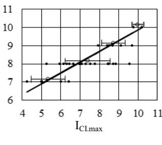
3-parameter; m=0.5933 n=3.9371; \(S_{\text{IMM}}\)=0.499 \(R^2\)=0.720
10-parameter; m=0.5933 n=3.9371; \(S_{\text{IMM}}\) =0.520 \(R^2\)=0.658
16-parameter; m=0.5933 n=3.9371; \(S_{IMM}\) =0.573 \(R^2\)=0.633
Figure 3. Plots between \(I_{MM}\) and \(I_{Cl.max}\) for 3-, 10-, and 16-parameters of the thirty-one earthquakes. Error bars of mean \(\pm\) sigma and the regression relations of \(I_{MM} = m I_{Cl.max} + n\) are indicated of period lengthening could increase the damage potential one scale-up for certain classes of structures. Structures with fundamental periods of, say, T=3.5seconds, would experience periods lengthening due to inelastic deformation and the soil-structure interaction to become, say, 4 seconds. This corresponds with an increase of one MMI scale from 9 to 10 due to period lengthening phenomenon (Katsanos et. al. 2014). Such an increase in MMI scale could not be predicted by the currently available methodologies.
The study was performed based on the limited earthquake data set listed in Table 1. The accuracy of the results could be further improved by considering more data, or more specific events focusing on a certain region. This is also the case for the relation shown in Figure 3 because the data in Table 1 merely considered earthquakes with intensity I<sub>MM</sub> ≥7. However, the methodology developed herein is still applicable.
8. Conclusion
Based on the investigations outlined above, the following conclusions can be drawn:
- 1. An alternative method to strong earthquake ground motion characterization was formulated. The characterization was based on the spectral acceleration, \(S_a(T)\), the significant duration, \(D_{05-95}\), and the peak ground velocity, PGV. They were computed based on three-component earthquake ground motions. Each of these three parameters correlated to 80% or higher with other parameters it represented. Altogether, the three parameters represented nine to ten other parameters of sixteen totally, or about 63%, resulting in a median value confidence level. The three parameters were combined to yield the composite-intensity index.
- 2. The index, I<sub>CI</sub>, was related to the modified Mercalli intensity, I<sub>MM</sub>, to assign its damage potentials. Thirtyone three-component earthquake records collected worldwide were studied. Among these earthquakes, the well-known Kobe 1995 (Takatori), New Zealand 2010, and Northridge 1994 were among the strongest earthquakes. The Mexico 1995 earthquake showed the most distinct character which could be more detrimental when considering the period elongation of structures.
- 3. Practical application to Chi-chi earthquake showed more meaningful interpretations of its characters. The damage potentials of Chi-chi showed that at a lower period than about 0.8 seconds it was perceived as 8 MMI; but it was 10 MMI for periods higher than 4 seconds; and 9 MMI in between them. It became critical at the transition periods as the period elongation due to inelastic response and soil-structure interaction might be an issue.
Acknowledgement
The authors acknowledged the support of the Engineering Centre for Industry and the Centre for Infrastructures and Built Environment, both of Institute of Technology Bandung. The authors also gratefully
acknowledged the constructive comments by the anonymous reviewer.
References
- Ang, A. H. S. and Tang, W. H. (2007) "Probability concepts in engineering: Emphasis applications in civil and environmental engineering," John Wiley & Sons.
- Arias A. (1970) "A measure of earthquake intensity," in Seismic Design for Nuclear Power Plants, ed. R. J. Hansen (MIT Press, Cambridge, MA), 438-
- Baker, J.W. and Cornell, C.A. (2006) "Which Spectral Acceleration Are You Using?," Earthq. Spectra, 22, 293-312.
- Bijukchhen, S., Takai, N., Shigefuji, M., Ichiyanagi, M. and Tsutomu, S.T. (2017) "Strong-Motion Characteristics and Visual Damage Assessment around Seismic Stations in Kathmandu after the 2015 Gorkha, Nepal, Earthquake," Earthq. Spectra, 33(S1), S219-S242.
- Bommer, J.J. and Martínez-Pereira, A., (1999) "The Effective Duration of Earthquake Strong Motion," J. Earthq. Eng., 3(2), 127-172.
- Bommer, J.J. and Alarcon, J.E. (2006) "The Prediction and Use of Peak Ground Velocity," J. Earthq. Eng., 10, 1-31.
- Bozorgnia, Y. and Campbell, K.W. (2004)"Engineering Characterization of Ground Motion," in Earthquake Engineering: From Engineering Seismology to Performance-Based Engineering, Bozorgnia, Y. and Bertero, V.V., Chapter 5, 215-315.
- Bradley, B.A. (2012) "Empirical Correlations between Peak Ground Velocity and Spectrum-Based Intensity Measures," Earthq. Spectra, 28, 17-35.
- Campbell, K.W. and Bozorgnia, Y. (2012) "Cumulative Absolute Velocity (CAV) and Seismic Intensity Based on the PEER-NGA Database," Earthq. Spectra, 28(2), 457-485.
- Elenas, A. (2000) "Correlation between Seismic Acceleration Parameters and Overall Structural Damage Indices of Building," Soil Dynam Earthquake Eng., 20, 93-100.
- Fajfar, P., Vidic, T. and Fischinger, M. (1990) "A measure of earthquake motion capacity to damage medium-period structures," Soil Dynam Earthquake Eng.,9(5), 236-242.
- Garcia, A.G. and Bernal, A.G. (2008) "Relationships Instrumental Ground between Motion Parameters and the Modified Mercalli Intensity in Guerrero, Mexico," 14th World Conference on Earthquake Engineering, Beijing, China.
- Ghobarah, A. and Elnashai, A.S. (1998), "Contribution of vertical ground motion to the damage of R/C buildings," Proceedings of the 11<sup>th</sup> European Conference on Earthquake Engineering, Balkema, 468-477.
- Goto, H. and Morikawa, H. (2012) "Ground motion characteristics during the 2011 off the Pacific Coast of Tohoku Earthquake," Soil Mech Found Eng., 52(5), 769-779.
- Hancock, J. and Bommer, J.J. (2006) "A State-of-Knowledge Review of the Influence of Strong-Motion Duration on Structural Damage," Earthquake Spectra, 22(3), 827-845.
- Housner, G.W. (1952) "Spectrum intensities of strongmotion earthquakes," Symposium on Earthquakes and Blast Effects on Structures, Los Angeles, CA.
- Katsanos, E.I., Sextos, A.G. and Elnashai, A.S. (2014) "Prediction of inelastic response periods of buildings based on intensity measures and analytical model parameters," Eng Struct., 71, 161-177.
- Luco, N. and Cornell, C. (2007), "Structure-Specific Scalar Intensity Measures for Near-Source and Ordinary Earthquake Ground Motions," Earthq. Spectra, 23(2), 357-392.
- Massumi, A. and Selkisari, M.R. (2017) "Correlations between Spectral Parameters of Earthquakes and Damage Intensity in Different RC Frames," Eng Geol., 11(3), 133-158.
- Medvedev, S.V. and Sponheuer, W. (1969) "Scale of Seismic Intensity," 4<sup>th</sup> World Conference Earthquake Engineering, Santiago, Chile, A-2, 143-153.
- Mylonakis, G. and Syngros, C. (2004), "The Collapse of Fukae (Hanshin Expressway) Bridge, Kobe, 1995: The Role of Soil and Soil-Structure Interaction," International Conference on Case Histories in Geotechnical Engineering, 12.
- PEER (2020) "Ground Motion Database," Pacific Earthquake Engineering Research Center.
- Perrault, M. and Guéguen, P. (2015), "Correlation between Ground Motion and Building Response Using California Earthquake Records," Earthq. Spectra, 31(4), 2027-2046.
- Sandeep, G.S. and Prasad, S.K. (2012) "Housner Intensity and Specific Energy Density for Earthquake Damage Assessment from Seismogram," Proceedings of International Conference on Advances in Architecture and Civil Engineering, Karnataka, India.
- Trifunac, M.D. and Brady, A.G. (1975) "A Study on Duration of Strong Earthquake Ground
- Motion," Bulletin of the Seismological Society of America, 65, 581-626.
- Von Thun, J., Roehm, L., Scott, G., Wilson, J. (1988) "Earthquake Ground Motions for Design and Analysis of Dams", Earthquake Engineering and Soil Dynamics II-Recent Advances in Ground-Motion Evaluation, Geotechnical Special Publication, 463-481.
- Wald, D. J., Quitoriano, V., Heaton, T. H. and Kanamori, H. (1999) "Relationships between peak ground acceleration, peak ground velocity, and Modified Mercalli Intensity in California," Earthq. Spectra, 15, 557–564.
- Wood, H.O. and Neumann, F. (1931) "Modified Mercalli Intensity Scale of 1931," Bull Seismol Soc Am., 21(4), 277-283.
- Wu, H., Masaki, K., Irikura, K., Saguchi, K., Kurahashi, S. and Wang, X. (2012) "Relationship between Building Damage Ratios and Ground Motion Characteristics during the 2011 Tohoku Earthquake," J. Natural Disaster Science, 34(1), 59-78.
- Wu, Y.M., Teng, T.L., Shin, T.C. and Hsiao, N.C. (2003) "Relationship between Peak Ground Acceleration, Peak Ground Velocity, and Intensity in Taiwan," Bull Seismol Soc Am., 93, 386-396.
- Xie, J., Wen, Z. and Li, X. (2012), "Characteristics of Strong Motion Duration from the Wenchuan M<sub>w</sub> 7.9 Earthquake," 15<sup>th</sup> World Conference on Earthquake Engineering, Lisboa.
- Zhang, Y., He, Z. and Yang, Y. (2018) "A Spectral-Acceleration-Based Linear Combination-Type Earthquake Intensity Measure for High-Rise Buildings," J. Earthq. Eng., 22(8), 1479-1508.