
1. Introduction
The Bogowonto River is the main river in the Bogowonto watershed which is included in the Serayu Bogowonto River Area, which has an area of ± 7,370.74 km2 and as many as 15 watersheds that flow from the slopes of Mount Sumbing (3,375 m msl) Wonosobo Regency, Purworejo City, Central Java Province to the estuary in Temon District, Kulonprogo Regency, Yogyakarta Special Region Province. The Serayu Bogowonto WS, which is prone to flooding, is the downstream area, which is primarily an agricultural area (Ningrum, 2014). Downstream of the Serayu Bogowonto WS is one of the potential areas, so it is a national strategic area due to the development of tourism supporting facilities, especially in the Yogyakarta area and its surroundings. However, this potential causes land-use change, resulting in erosion and sedimentation downstream (Suprapto, 2015).
In the dry season, the mouth of the Bogowonto river closes because sediment deposits accumulate at the river mouth, disrupting the river flow to the sea (Bambang, 1999). At high tide, sediment holds the Bogowonto river flow because it impacts the backwater downstream of the Bogowonto river, causing flooding in several locations, especially around Yogyakarta International Airport. On the west side of the estuary of the Bogowonto River, it has been developed into a mangrove tourism area. The east side of the estuary has become a protected area for YIA (Yogyakarta International Airport) (Neneng, 2019). At the mouth of the Bogowonto River, a jetty was built in 2008, but the condition was damaged and covered by sediment, so it needed to be rebuilt.
2. Study Area
The research did in the Bogowonto River Basin (DAS), especially downstream to the mouth of the Bogowonto river in Kulon Progo Regency, D.I Province. Yogyakarta.
3. Materials and Method
3.1 Hydrology
In this subchapter, the delineation of the Bogowonto watershed has been carried out where the catchment area is 572,194 km<sup>2</sup>. Then proceed with finding the area of influence of the rain station using Thiessen Polygon.
The data used is the maximum annual rainfall data for 20 years from 2000 - 2019 in the Bogowonto watershed, including three rain stations, namely Jogoboyo Rain Station, Penungkulan Rain Station, and Sapuran Rain Station. Rainfall analysis was carried out using several methods such as normal distribution, Gumbel, Log-Normal, and Log Pearson Tipe III (Chow, at al., 1988). The data is analyzed in rainfall, and the regional rainfall is calculated. The value of regional rainfall is calculated using a synthetic unit hydrograph to produce a
Figure 1. The jetty condition that has been damaged and covered in sediment.
design discharge. Based on the rainfall distribution during these hours, a flood hydrograph modeling for the Bogowonto watershed was carried out. This study used Nakayasu Hydrograph, SCS Hydrograph, ITB-1b Hydrograph, and ITB-2b Hydrograph for each return period (Natakusumah, at al., 2011). Calibration was carried out with flood discharge data from Boro Dam (Pawestari, Istiarto, 2016) from 2000 to 2019 (Table 1).
The frequency analysis results of the observed flood discharge were compared with the results of the flood discharge from the hydrograph model (Figure 4).
For flood simulation modeling as flood control in the YIA Airport area, Q100 is used (Puspa, Purwono,
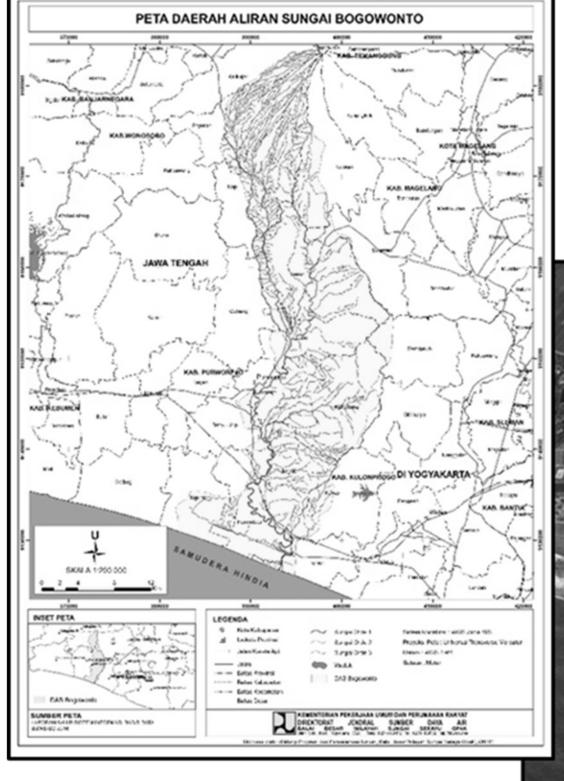
Figure 2. Study area
Table 1. Peak discharge each return period.
| Return Period (Year) | Discharge Observation Data (m³/s) | Nakayasu (m³/s) | SCS (m³/s) | ITB-1b (m³/s) | ITB-2b (m³/s) |
|---|---|---|---|---|---|
| 2 | 859.72 | 718.02 | 648.25 | 653.05 | 687.83 |
| 5 | 1151.29 | 925.99 | 845.91 | 852.62 | 890.81 |
| 10 | 1304.02 | 1064.34 | 977.41 | 985.39 | 1025.82 |
| 25 | 1453.27 | 1241.07 | 1149.64 | 1159.64 | 1199.08 |
| 50 | 1571.29 | 1372.88 | 1279.58 | 1291.23 | 1328.57 |
| 100 | 1668.48 | 1503.72 | 1408.56 | 1421.83 | 1457.10 |
| 200 | 1755.26 | 1634.07 | 1537.07 | 1551.97 | 1585.16 |
| 1000 | 1932.28 | 1936.03 | 1834.76 | 1853.41 | 1881.81 |
Figure 3. Watershed of Bogowonto river and thiessen polygon.
2020). By setting the parameter alpha (\(\alpha\)) value, the closest hydrograph is HSS Nakayasu with \(\alpha\) =2. A reliable flow will be calculated using the NRECA Method with a data range from 2010-2019, calibrated using the AWLR Pungangan Data (Figure 5).
So, hydrology analysis shows that the average discharge is \(19.2 \text{ m}^3/\text{s}\). On the other side, discharge of wet season and dry season in order are \(26.5 \text{ m}^3/\text{s}\) and \(11.8 \text{ m}^3/\text{s}\).
3.2 Hydro-oceanography
Analyzing tides is using the data from Delft Dashboard. Parameter of the tide can be downloaded in that software. The boundary of parameter data is based on Boundary Condition (TPXO 7.2 Global Inverse Tide Model) (Mardika, 2020). The tidal model data obtained were processed using Delft3d-TIDES for 15 days from 12-26 August 2019, calibrated using BIG data.
In analyzing wave hindcasting, the wind data used is Copernicus wind data for ten years, namely in 2011-2020. The hindcasting method used is the 1984 Shore Protection Manual (SPM) method. In addition to wind
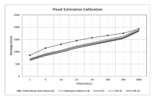
Figure 4. Flood peak discharge calibration
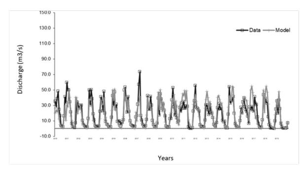
Figure 5. The calibration between calculation and observation discharge.
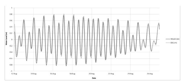
Figure 6. The calibration between Delft3D tides modelling and observation tides (BIG).
data, wave hindcasting requires data fetch as hindcasting input (Pokaton, 2013). From the results of the hindcasting analysis, the dominant wave distribution
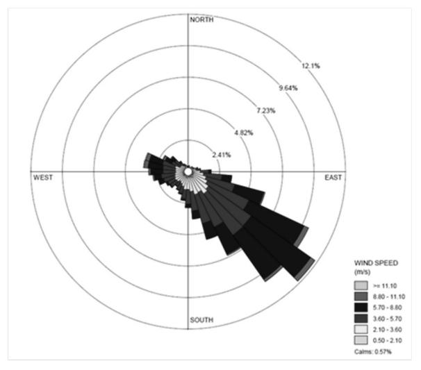
Figure 7. Significant wave rose
in the wet season comes from the west. Meanwhile, the dominant wave is from the southeast in the dry season, for the distribution of the dominant significant wave from the southeast direction is described in Figure 7.
Thus, the result of wave analysis is a significant wave direction from the southeast with a significant wave height of 3.34 m and a wave period of 11.11 seconds.
3.3. Methodology
This research's flowchart is shown in down below Figure 8.
4. Result and Discussion
4.1. Hydrolic modelling
This modeling used two scenarios in scenario one where the capacity of the estuary is closed, and there is no jetty. In scenario two, the condition is when the capacity of the estuary is open, and a jetty has been built (Baskoro,2009). The scenario with the jetty building has the right and left jetty lengths of 300 m according to the design drawings built (Figure 9).
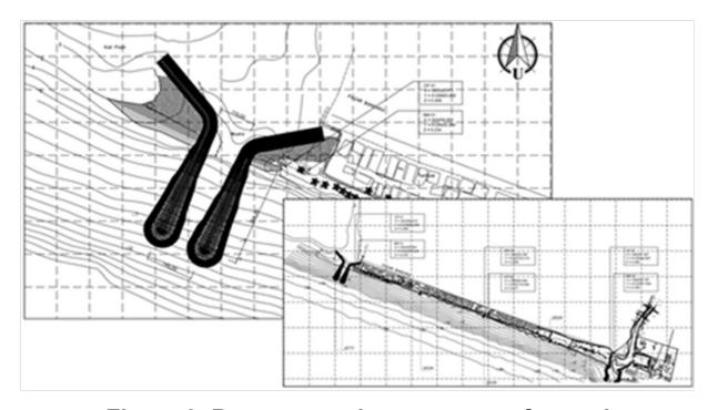
Figure 9. Bogowonto river estuary safeguard design layout
Using the Manning Formula with the assumption of uniform flow, an analysis can be carried out to determine the manning value in the river using hydrometric data (flow and river area) and topographic data (slope of the riverbed) (Prhyuono, 2011). From the calculation results, the average Manning coefficient value = 0.03. Both scenarios are simulated using a flow hydrograph (upstream) from Q100 flood discharge data for YIA Airport flood control design from hydrological calculations and using Highest High Water Level (HHWL) and significant wave height (Hs) data as a stage hydrograph (downstream). So that the results of the flood modeling for the two scenarios can be seen in the following Figure 10 and 11.
The simulation results of scenario 1 resulted in a water level rise of about 1 m from the estuary. It had a backwater impact up to a distance of about 2.9 km from the Bogowonto estuary. With elevation
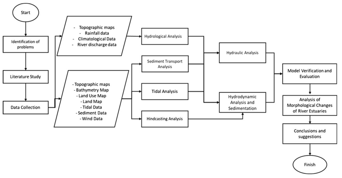
Figure 8. Flowchart.
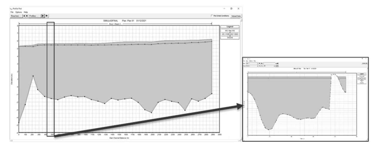
Figure 10. Simulation of the lower estuary flood of Bogowonto river and cross section STA-400 scenario 1
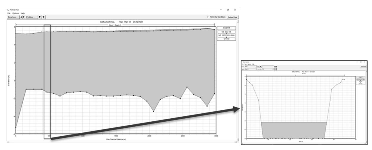
Figure 11. Simulation of the lower estuary flood of Bogowonto river and cross section STA-400 scenario 2
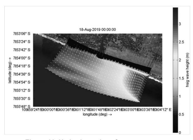
Figure 12. Hydrodynamics of ocean waves to the Bogowonto river estuary
modification using Jetty design and normalization (300m from the estuary) for scenario 2, it results in a change in water level rise due to backwater to 0.2 m, so scenario two conditions can reduce water level rise to scenario one by about 0.8 m.
4.2. Hydrodynamic modelling
From calculating the height and period of significant waves (Hs and Tp) and the direction of the waves from the wind data, hydrodynamics can be simulated using Delft3d-WAVE to see the direction of the waves and their effect on the coast. Simulations were carried out for one day every 1-hour using data from significant waves and tides at full moon.
From the simulation results, it can be that the sea waves have a height of about 2 - 3.5 m. When the wave reaches the estuary, the sea wave has a height of about 1 -2 m, coming from the southeast. The waves tend to travel along the shoreline, which can cause longshore sediments (Chrysanti, Adityawan, 2019).
4.3. Transport sediment modelling
The modeling was carried out for 15 days, and the input value of the Morphological Scale Factor (MOR) was 24. Thus, the modeling carried out for 15 days would equal 360 days (±1 year) (Suryadi, 2020).
Erosion and sedimentation modeling was carried out in two different scenarios, namely West Side Jetty (300 m) + East Side (300 m) for scenario one, and West Side Jetty (300 m) + East Side (400 m + 300 m Southwest Direction) for scenario two which is inputted to the dry points as the Jetty model. The following are the modeling results for Scenario one and Scenario two.
When modeling Scenario one using a parallel jetty, sedimentation occurs at the end of the jetty to a height
Table 2. Transport sediment modeling input data
| Parameter | Parameter Value | |
|---|---|---|
| Bogowonto watershed discharge (average) | 19,2 m3 /s | |
| Significant Wave | ||
| Hs | 3,34 m | |
| Ts | 11,11 s | |
| Direction | Southeast | |
| Sediment | ||
| D50 | 410 µm | |
| TSS Bogowonto River Estuary | 0,001 kg/m3 | |
| Morphological Scale Factor (MOR) | 24 | |
| Modeling Duration | 15 Days | |
of 3 m to cover the mouth of the Bogowonto river estuary. Meanwhile, in Scenario two, sedimentation occurs on the east side of the jetty, but the mouth of the Bogowonto river estuary remains open.
4.4. Morphological changes modelling
Delft3d FLOW – WAVE modeling that has been run obtained the results of changes in river and coastal morphology (Mallick, at al., 2018) that occur around the mouth of the Bogowonto river based on Scenario 1 and Scenario 2. For scenario 1, Jetty modeling for West Side (300 m) + East Side (300 m) was carried out. For scenario 2, jetty modeling for the West Side (300 M) + East Side (400 M + 300 m Southwest Direction) is carried out. The following are the morphological changes modeling results for Scenario one and Scenario two.
In scenario 1, with parallel jetty conditions, the estuary's mouth has relatively large sedimentation. It covers the entire mouth of the estuary and can inhibit the flow of the Bogowonto river discharge during the rainy season, which can cause flooding. Morphological changes that occur on the east side of the Bogowonto
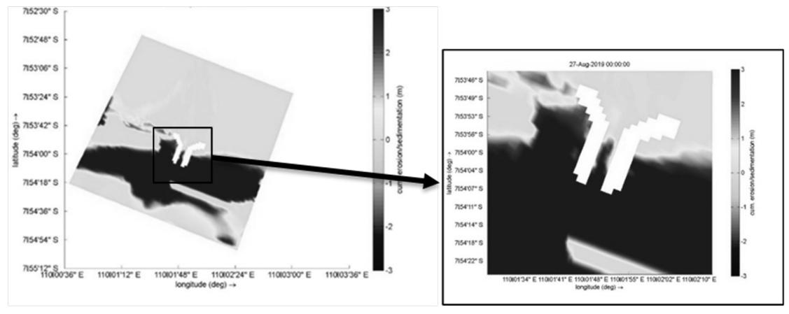
Figure 13. Erosion and sedimentation modeling scenario 1
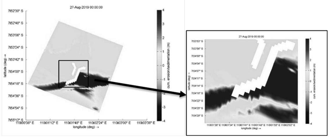
Figure 14. Erosion and sedimentation modeling scenario 2
Figure 15. Morphological changes modeling scenario 1
Figure 16. Morphological changes modeling scenario 2
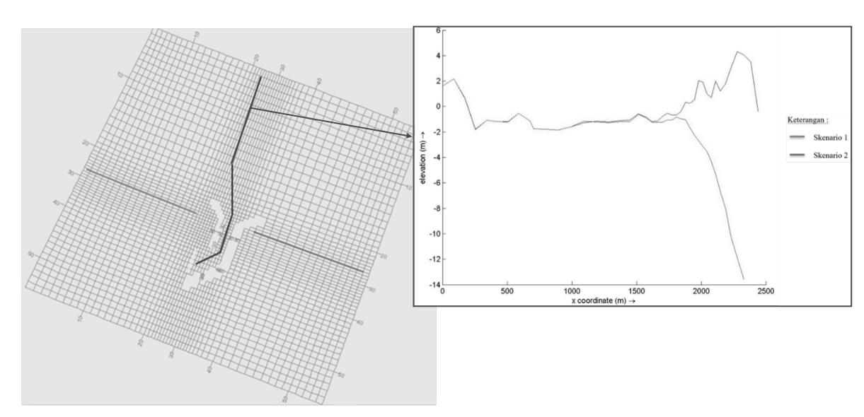
Figure 17. Morphological changes modeling scenario 2
River Estuary result from sedimentation, which causes the coastline to move forward 5 m for one year.
In scenario 2, with a longer jetty on the east side, the mouth of the estuary is open so that the discharge of the Bogowonto river during the rainy season can flow. Morphological changes on the east side of the Bogowonto River Estuary result from sedimentation, which causes the coastline to move forward 6 m for one year. But there is potential for erosion to the east (Glagah Beach) for one year as far as 1 m.
Based on the simulation results, it can be seen that there are differences in changes in riverbed elevation in scenario one and scenario 2 in 1 year. Figure 17 is a graph of the different changes in river bed elevation taken from the Grid in Delft3D Quickplot.
Based on Figure 17, Scenario 1 tends to experience sedimentation while Scenario 2 does not experience sedimentation in the estuary. This condition is because the Jetty in scenario two can hold sediment carried by significant waves from the southeast compared to scenario 1.
5. Conclusion
The conclusions obtained to fulfill the aims and objectives are:
- 1. Flood discharge during Q100 return with HSS Nakayasu is 1503.72 m3/s. The mainstay discharge (Monthly) was calculated on the Bogowonto river using the NRECA method. The average value is 19.2 m3/s. The results of the tidal analysis obtained the Highest High Water Level (HHWL) value of 1.901 m. The hindcasting analysis results obtained a significant wave (Hs) up to the mouth of the Bogowonto river of 3.34 m which was dominated from the southeast.
- 2. The simulation results of the flood modeling in the Lower Bogowonto River when the estuary is closed give a backwater impact up to a distance of about 3 km with a water level rise of about 1 m. When the estuary is open and there is a jetty, the change in water level rises due to backwater becoming 0.2 m. If normalization is carried out and the jetty in the estuary, the water level is reduced by about 0.8 m.
- 3. Simulation of changes in the morphology of the river estuary was carried out in 2 scenarios, where the results for Scenario 1 still have the potential to have a sedimentation impact at the end of the jetty so that it can close the flow of river discharge. In contrast, Scenario 2 can overcome the impact of sedimentation so that the Bogowonto river can be flow discharged into the sea. This condition is because the jetty in scenario two can hold sediment carried by significant waves from the southeast compared to scenario 1.
References
- Baskoro Wursito Adi 2009. Kajian Pengaruh Pembangunan Jetty Terhadap Kapasitas Sungai Muara Way Kuripan Kota Bandar Lampung.
- Chow V T et al 1988. Applied Hydrology, Mc Graw Hill Book Company, Singapore.
- Chrysanti A, Adityawan M B, et al. 2019. Prediction of Shoreline Change Using a Numerical Model: Case of the Kulon Progo Coast, Central Java. MATEC Web of Conferences 270(1):04023.
- Dibyosaputro Suprapto 2015. Morphometry Characteristics of Riverbed Sediment Grains as Basic Indicator Management of River Valley Environment (Case Study of Bogowonto River, Central Java).
- Fahmi Mirza T, Hafli Mudi 2019. Simulasi Numerik Perubahan Morfologi Pantai Akibat Konstruksi Jetty pada Muara Lambada Lhok Aceh Besar Menggunakan Software DELFT3D.
- Mardika M Gilang Indra 2020. Study Of Sediment Control In The Bogowonto River Estuary, Kulon Progo, Province Of Daerah Istimewa Yogyakarta.
- Natakusumah D K, Hatmoko W and Harlan D 2011. General procedure for calculating synthetic unit hydrograph by ITB method and some examples of its application in Civil Engineering Journal 18 251-291(In Bahasa).
- Ningrum M 2014. Kajian Perubahan Penggunaan Lahan DAS Bogowonto terhadap Rencana Tata Ruang Wilayah Dalam Rangka Pengendalian Sedimentasi. Universitas Gadjah Mada. Yogyakarta. Corpus ID 131689841.
- Pawestari Margareth Titi, Istiarto. 2016. Flood Hazard Mapping of Bogowonto River in Purworejo Regency, Central Java.
- Pokaton Kern Youla 2013. Perencanaan Jetty di Muara Sungai Ranoyapo Amurang.
- Prhyuono Endy 2011. Effect of Jetty Construction Towards Water Elevation in Rejoso River Estuary, Pasuruan, Indonesia.
- Puspa Festi Windira, Purwono Novi Andhi Setyo 2020. Analisis Kondisi Muara Terhadap Banjir di Sungai Serang Kabupaten Kulonprogo.
- Rimayanti Neneng 2019. Perencanaan Sistem Drainase Sisi Darat Bandara New Yogyakarta International Airport (NYIA) di Kecamatan Temon, Kabupatern Kulon Progo, Daerah Istimewa Yogyakarta.
- Suryadi Yadi 2020. Kajian Sedimentasi di Muara Sungai Ciletuh, Kabupaten Sukabumi.
- Triatmodjo Bambang 1999. Teknik Pantai. Beta Offset. Yogyakarta.