
Abtsrak
Kali Dadap sering mengalami banjir di bagian muara. Kali Dadap terletak di Kecamatan Kosambi, Kabupaten Tanggerang. Permasalahan banjir di Kali Dadap disebabkan oleh berkurangnya kapasitas sungai dan muara yang disebabkan oleh sedimentasi dan pengaruh oleh kondisi pasang pasang surut. Banjir yang terjadi menyebabkan rusaknya prasarana kota serta melumpuhkan aktivitas warga yang terdampak. Kali Dadap telah dilakukan normalisasi pada tahun 2012 untuk mengatasi permalahan banjir yang terjadi. Tujuan dari studi ini yaitu untuk mengetahui kapasitas kali dan muara Dadap serta sebagai alternatif solusi penanganan banjir. Simulasi pemodelan banjir dilakukan pada kondisi sebelum dan sesudah dinormalisasi serta dengan alternatif peninggian tanggul. Pemodelan banjir dilakukan menggunakan aplikasi HEC-RAS 1D aliran unsteady. Pemodelan akan dilakukan dengan kondisi batas di bagian hulu menggunakan debit banjir dengan kala ulang 50 dan 100 tahun dan di bagian hilir menggunakan elevasi HHWL dan tinggi gelombang. Hasil analisis menunjukkan bahwa kapasitas Kali Dadap sebelum di normalisasi tidak mampu mengalirkan debit banjir kala ulang 50 dan 100 tahun. Setelah dilakukan normalisasi pada Kali Dadap, elevasi muka air dapat menurun sekitar 24 -29% tetapi masih terjadi banjir pada bagian hilir akibat pasang surut sehingga perlu adanya peninggian elevasi tanggul yaitu +3.5 m.
Kata Kunci: Kali Dadap, muara Dadap, banjir, normalisasi, HEC-RAS
1. Introduction
The northern coastal area of Jakarta is the estuary of rivers that originate in the southern region, including artificial canals. The rivers that flow into Jakarta Bay have a severe problem, with high sedimentation rates and flooding problems.
Dadap River is one of the rivers that flow towards into Jakarta Bay which often experiences flooding in the estuary. Dadap River is located in Kosambi District, Tangerang Regency, Banten Province, and is also the outlet of Soekarno Hatta Airport. The estuary of the river functions as a place for river discharge, especially during floods into the sea. The problem of flooding in the Dadap River is caused by the lack of rivers capacity and estuaries caused by sedimentation. In addition to these problems, the flood in the Dadap River is influenced by tidal conditions. Some of the flood events can be seen in Figure 1. The flooding that
Figure 1. Floods in Dadap Village, Kosambi District, Tangerang Regency, Banten Source: (a) metro.tempo.co, (b) republika.co.id, (c) antaranews.com
occurred caused damage to city infrastructure and paralyzed the activities of the affected residents. The Dadap River was normalized in 2012 to overcome the flooding problems. This study aims to determine the capacity of the Dadap river and estuary and as an alternative solution for flood management. Flood modeling simulations were carried out on the Dadap river and estuary in conditions before and after normalization (Sukmajari, at al., 2021) and alternative embankment elevations (Giyanto, at al., 2021). The alternative of raising the embankment considers land subsidence (Moe, at al., 2017) and climate change which causes increasing flood inundation areas, depths (Mishra, at.al., 2017), and sea-level rise (Mimura, 2013).
The study of flood control on the Tanggul River uses Hecras software with 1D modeling (Moe, at al., 2017). However, according to the HEC-RAS Manual, Hecras cannot model waves. In the study of sedimentation at the Ciletuh estuary, the waves were modeled using Delf3D (Suyadi, at, al., 2019). For the Dadap River itself, there has been no special study, so in this study a combination of HECRAS and Delft3D was used.
2. Materials and Methods
2.1 Data collection
The data used in the analysis were obtained from various sources. These data include the following.
· Topographical Data
Topographic data were obtained from Ciliwung Cisadane Major River Basin Organization. The topographic data used are in conditions before and after normalization.
· Rainfall data
Rainfall data used is GPM satellite rain data obtained from the website https://giovanni. gsfc.nasa.gov/giovanni/. Rain data was used from 2001-to 2020. Satellite data is used as an alternative for providing rainfall data. GPM satellite rainfall data was chosen because it has an excellent spatial resolution of 0.1o or 11.32 km (Technical Engineering Center for DAM, 2017).
· Tidal Data
Tidal data is needed to determine important elevations. The data will be used for analysis as the downstream boundary in the modeling. Tidal data was obtained from Geospatial Information Agency (BIG).
· Wind Data
Wind data is obtained from the Meteorological, Climatological, and Geophysical Agency (BMKG) website http://dataonline.bmkg.go.id/. Wind data used is hourly data for the years 2011-2020. Wind data is used for waves forecasting at the study site.
2.2. Hydrological analysis
Design rainfall was analyzed using satellite rainfall data. Satellite rainfall data is corrected against the Soekarno Hatta meteorological station. Inspection of GPM monthly rain data with the rain post aims to see the quality of monthly rain data. Data can be used if the correlation value is more than 0.6 and RMSE with a 58-84 for the monsoon rain pattern area (Mamenun, 2014). Rainfall analysis was carried out using several methods such as normal distribution, Gumbel, log normal, and log Pearson (Chow, et al., 1988). The compatibility test of the frequency distribution analysis used the Smirnov Kolmogorof and Chi-Square tests (Triatmodjo, 2008). The results of the design rainfall analysis are verified using an isohyet map (Yeh, at al., 2011) from the Director-General of Water Resources, Ministry of Public Works and Housing. The design flood discharge for the return period was analyzed using the Nakayasu, SCS, Snyder (Hec-HMS), ITB1b, and ITB2b (Natakusumah, at al., 2011) synthetic hydrograph methods following SNI 2415-2016 (National Standardization Agency, 2016). The design flood discharge is calibrated using a Creager curve (A Kang, at al., 2011).
2.3 Tidal analysis
The tidal analysis is calculated using the harmonic analysis method with the help of Delft3D software.
2.4 Wave analysis
The method used to calculate the significant wave height (Hs) and wave crest period (Ts) is the 1984 SPM method (CERC, 1984). The wave propagation from the sea to the river mouth is modeled using Delft3D software.
2.5 Hydraulic analysis
Hydraulic analysis was carried out for modeling flood conditions in the study area using HEC-RAS software version 5.07 for 1D unsteady flow type. HEC-RAS contains one-dimensional river analysis components for unsteady flow simulation (one-dimensional hydrodynamic) (US Army Corps of Engineers, 2016). Hecras cannot model waves, so the waves generated by Delft3D modeling are simplified as downstream boundaries along with the tides.
Based on the Ministry of Public Works & Housing Regulation Number 28 of 2015 (Minister of Public Works & Housing Regulation No 28 PRT/M/2015) concerning the Determination of River and Lake Border Lines, the Flood Embankment Design must comply with the provisions that the dimensions of the bank and embankment area are as follows: shown in Table 1.
Table 1. Criteria design flood discharge by region
| Criteria | Design flood Discharge | ||
|---|---|---|---|
| Capital of the District/City | (Q10 – Q20) | ||
| Capital of the Province | (Q20 – Q50) | ||
| The nation's capital /Metropolitan | (Q50 – Q100) | ||
According to the Ministry of National Development Planning, the Republic of Indonesia, Tanggerang Regency, and Tangerang City are metropolitan areas in the list of metropolitan areas, so the design flood discharges of Q50 and Q100 are used. The flood modeling simulation uses the layout and boundaries shown in Figure 2.
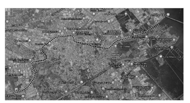
Figure 2. Geometry layout modeling for the Dadap River flood
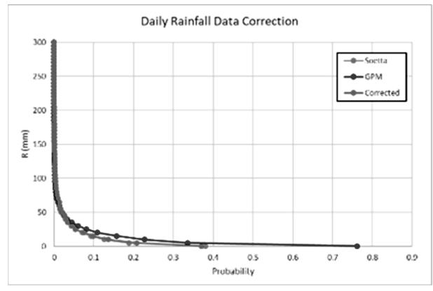
Figure 3. Satellite daily rain data correction
The boundary conditions used in this modeling include:
- · Boundary upstream uses design flood discharge for 50 and 100 year return periods,
- · Downstream Boundary using constant HHWL based on tidal analysis and Wave Height.
- · Modeling carried out for 48 hours.
- · The manning roughness value used is 0.059-0.062 for conditions before normalization and 0.01-0.024 for conditions before normalization. The manning value was obtained based on the results of the calibration of the instantaneous discharge value from the measurements in the field.
Modeling scenario:
- · Conditions before and after normalization using design flood discharge for a Q100 year return period.
- · Conditions before and after normalization using design flood discharge for a Q100 year return period.
- · Conditions after normalization + embankment elevation using design flood discharge for Q50 and Q100 year return periods.
3. Results and Discussion
3.1 Hydrological analysis
3.1.1 Correction of satellite rain data
Satellite rainfall data is corrected against the Soekarno Hatta rain station. Correction factors for daily rain data are carried out by trial and error on rain data in the field. Figure 3 shows a graph of the probability of corrected daily rainfall. Based on the results of the corrections, satellite rain data can be used (Mamenun, 2014) and get a correlation value with a high degree of association, namely 0.8545, an RMSE value of 81.1402 (for the monsoon rain pattern area, the RMSE value is between 58-84), and meets the NSE value of 0.7091. Comparison of monthly rainfall data from satellite rain, corrected data, and ground station can be seen in Figure 4.
3.1.2 Analysis of design rainfall
The results of the design rainfall analysis after being multiplied by the area reduction factor (ARF) following SNI 2415-2016 can be seen in Table 2. The compatibility
Table 2. The results of the design rainfall
| Return Period (T) (year) | Design Rainfall (mm) | |||||
|---|---|---|---|---|---|---|
| No | Normal | Gumbel | Log Normal | Log Pearson III | ||
| 1 | 2 | 118.2 | 110.2 | 109.3 | 109.1 | |
| 2 | 5 | 159.0 | 153.1 | 153.9 | 153.8 | |
| 3 | 10 | 180.4 | 181.5 | 184.0 | 184.1 | |
| 4 | 25 | 203.2 | 217.4 222.7 | 223.5 | ||
| 5 | 50 | 217.9 | 244.1 | 251.9 | 253.3 | |
| 6 | 100 | 231.2 | 270.5 | 281.4 | 283.6 | |
| Smirnov Kolmogorof test | 0.135 | 0.089 | 0.115 | 0.098 | ||
| 0.270 0.270 | 0.270 | 0.270 | ||||
| accepted accepted accepted | accepted | |||||
| Chi-Square test | 3.400 | 6.400 | 4.600 | 4.600 | ||
| 7.815 | 7.815 | 7.815 | 7.815 | |||
| accepted | accepted | accepted | accepted | |||

Figure 4. Comparison of monthly rainfall data from satellite rainfall, Soekarno Hatta, and corrected satellite rainfall data
test results of frequency distribution analysis, Gumbel, and Log Pearson III methods have the best results. Then it is compared with the isohyet map from the Director-General of Water Resources (Figure 5). R100 on the isohyet map is around the 250-275 rain contour. Based on the compatibility test results and verification of the isohyet map (Yeh, at al., 2011), the design rainfall was chosen using the Gumbel method. The selected design rainfall is 244.05 mm for the 50-year return period and 270.49 mm for the 100-year return period.
3.1.3 Analysis of design flood discharge
Dadap river does not have discharge data, and the cross -section of the river has been normalized and is not natural, so calibration is carried out using a Creager curve. The results of the analysis design flood
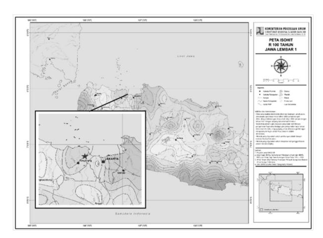
Figure 5. Ishoyet R100 map of the study area source: Ministry of Public Works & Housing
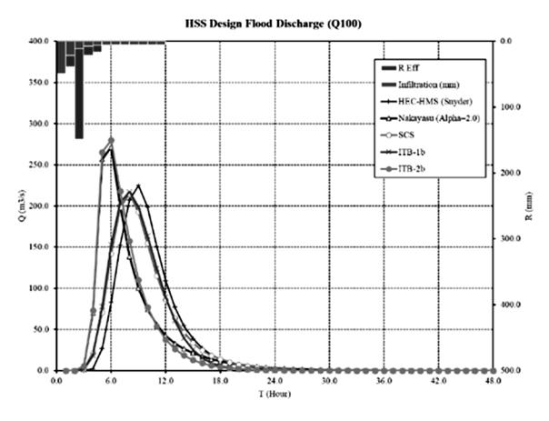
Figure 6. HSS design flood discharge with several methods (Q100)
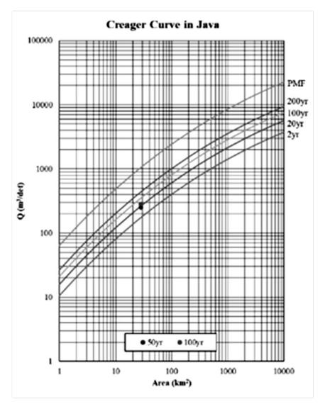
Figure 7. Calibration of the design flood discharge on the creager curve
Table 3. The results of return period design flood discharge with several methods
| Design Flood Discharge (m3 /s) | ||||||
|---|---|---|---|---|---|---|
| Tr | Nakayasu | SCS | Snyder | ITB-1b | ITB-2b | |
| 2 | 97.62 | 75.37 | 79.00 | 76.01 | 100.42 | |
| 5 | 144.21 | 112.69 | 118.10 | 113.85 | 148.48 | |
| 10 | 175.06 | 137.40 | 144.00 | 138.90 | 180.30 | |
| 25 | 214.04 | 168.63 | 176.80 | 170.55 | 220.50 | |
| 50 | 242.95 | 191.79 | 201.00 | 194.03 | 250.32 | |
| 100 | 271.65 | 214.78 | 225.10 | 217.34 | 279.92 | |
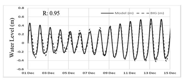
Figure 8. Validation tidal time series
Table 4. Tidal analysis results
| Chart Datum (m) | |||
|---|---|---|---|
| Important Elevation Values | MSL | LLWL | |
| Highest High Water Level (HHWL) | 0.7879 | 1.5760 | |
| Mean High Water Level (MHWL) | 0.6729 | 1.4160 | |
| Mean Sea Level (MSL) | 0 | 0.7880 | |
| Lowest Low Water Level (LLWL) | -0.7881 | 0.0000 | |
| Lowest Astronomical Tide (LAT) | -0.8711 | -0.0830 | |
discharge with several methods can be seen in Table 3. The comparison of the HSS of the design flood discharge for each method is shown in Figure 6. Design flood discharge of the 100-year return period on the Creager curve is 350.82 m3 /s and then calibrated using a Creager curve (A Kang, at al., 2011), as shown in Figure 3. The result of the Q100 flood discharge
calculation closest to the Creager curve is the ITB-2b method, which is 279.92 m3 /s. So based on this calibration, the results of the analysis of the design flood discharge were chosen using the ITB-2b method.
3.2 Tidal analysis
Tidal forecasting using data in Muara Dadap validated with a model from Delft3D with the correlation value obtained is 0.95. Based on the results of the tidal
Figure 9. Length of fetch
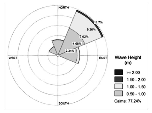
Figure 10. Waverose for the year 2011-2020 Figure 11. Wave propagation to the river mouth
analysis, the Formzhal number value is 2.4696 (mixed diurnal). The important elevation values from the analysis can be seen in Table 4. The hydraulic analysis will use the tidal elevation on the chart datum LLWL.
3.3 Wave analysis
Based on the results of wave forecasting, a significant wave height of 3.54 m was obtained with a wave period of 11.32 seconds from the northeast. The wave roses for 2011-2020 can be seen in Figure 10. Then the wave propagation from the sea to the Dadap estuary is modeled using Delft3D software with a wave height of 0.5 m, as shown in Figure 10.
3.4 Hydraulic analysis
3.4.1 Flood modeling in conditions before and after normalization
Based on the flood modeling results that have been carried out, the river's capacity before normalization cannot pass the Q100 flood discharge. The simulation results show that normalization can reduce the water surface elevation, but there are still some overflowing crosses, especially downstream. The water surface elevation was reviewed further on several critical cross-sections,
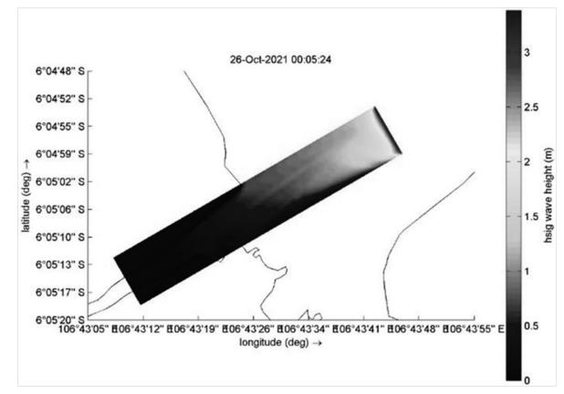
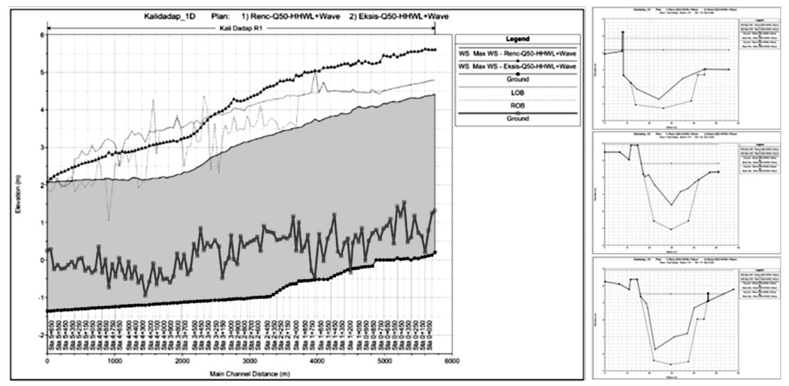
Figure 12. Results of flood modeling on conditions before and after normalization with Q50 years.
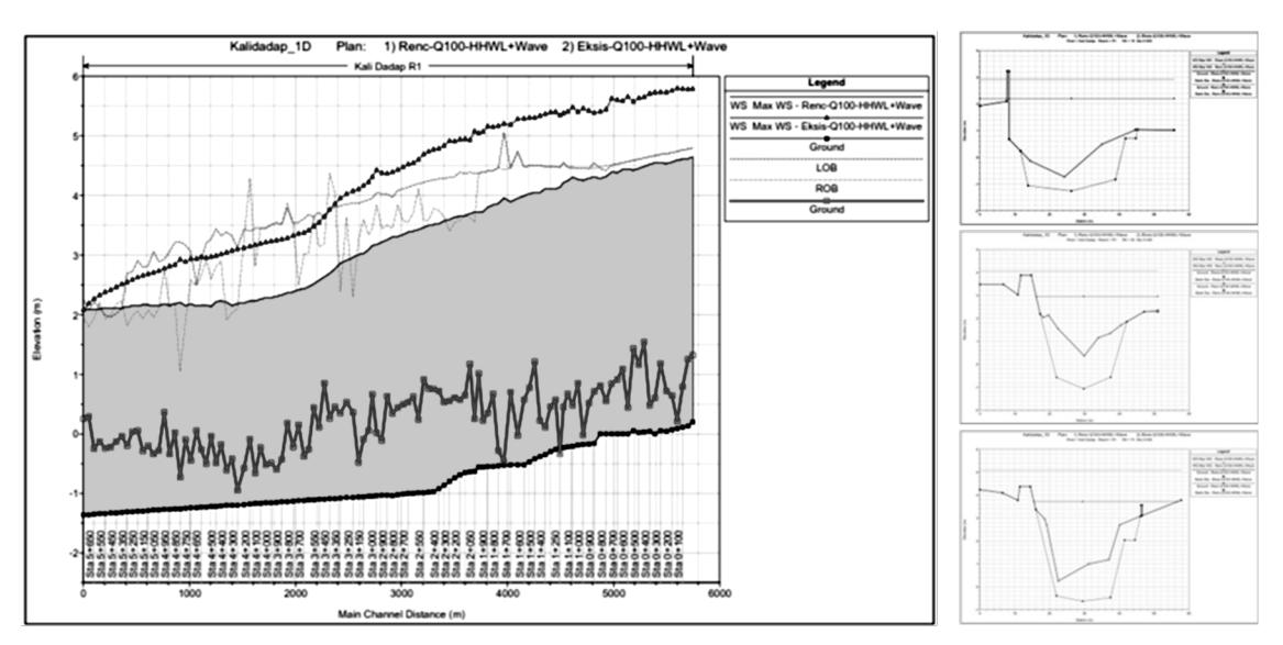
Figure 13. Results of flood modeling on conditions before and after normalization with Q100 years.
Table 5. Reduction of water surface elevation
| Cross | Water Surface Elevation (m) | |||||
|---|---|---|---|---|---|---|
| Q50 | Q100 | |||||
| Section | Before normalization (m) | After normalization (m) | Reduction (%) | Before normalization (m) | After normalization (m) | Reduction (%) |
| Cross 18 | 2.86 | 2.18 | 24% | 2.92 | 2.2 | 25% |
| Cross 50 | 3.94 | 2.81 | 29% | 4.07 | 2.96 | 27% |
| Cross 74 | 4.92 | 3.52 | 28% | 5.08 | 3.72 | 27% |
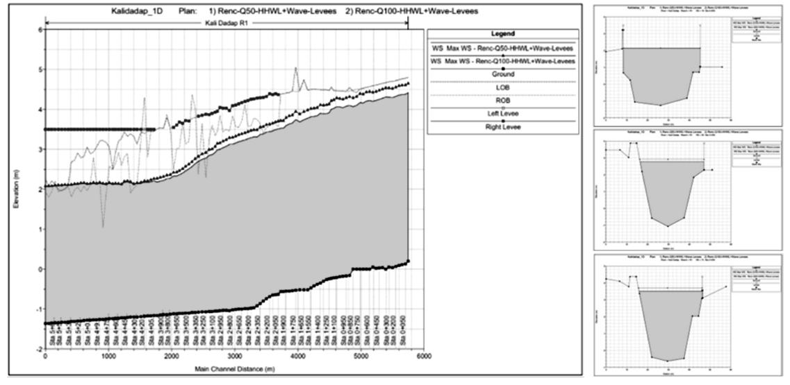
Figure 14. Flood modeling with normalization and embankment elevation.
namely Cross 18, Cross 50, and Cross 74. The flood elevation with Q100 discharge on the cross fell around 0.68 – 1.4 m or around 24-29%, as shown in Figure 12. Meanwhile, the flood elevation with Q50 discharge on the cross decreased by about 0.72 – 1.36 m or about 25-27%, as shown in Figure 13. The water surface elevation review summary can be seen in Table 5.
3.4.2 Flood modeling after normalization and embankment elevation
Based on the flood modeling results, overflow still occurs downstream after normalization. Some embankments on the right side also have an overflow, such as cross 48, cross 50, cross 68 and cross 74.
Therefore, it is necessary to raise the embankment elevation. The elevation of the downstream embankment refers to the flood modeling results. The upstream boundary with Q100 discharge and the downstream boundary in the form of HHWL and wave height, and considers land subsidence of 75 mm/year, sea-level rise of 8 mm/year (PT. Raya Konsult - KSO, 2016), and freeboard of 0.6 m, so that the elevation embankment downstream to +3.5 m. There is no embankment on the right side of the river from cross 40 to cross 74, so it is necessary to have an embankment with the same elevation as the left embankment. The flood problem in Dadap River can be overcome by structural measures: normalization and embankment elevation, as shown in Figure 14.
4. Conclusion
Based on the results of the analysis that has been carried out, the following conclusions are obtained.
- 1. The capacity of the Dadap River before normalization was not able to accommodate the design flood discharge at the 50 and 100 yr return periods.
- 2. After the normalization of the Dadap River, the water surface elevation may decrease by 24-29%, but there is still flooding downstream due to the tides.
- 3. It is necessary to raise the embankment elevation of +3.5 m downstream to overcome flooding due to tides.
Reference
- A Kang, Boo-Sik & Ryu, Seung-Yeop. 2011. Estimation of Probable Maximum Flood by Duration using Creager Method. Journal of Korean Society of Hazard Mitigation 11. 77-84.
- CERC 1984. Shore Protection Manual Volume I-II. US Army Corps of Engineers Washington DC.
- Chow, V T, et al. 1988. Applied Hydrology, Mc Graw Hill Book Company, Singapore.
- Giyanto, Harlan, D, and Natasaputra, S 2021. Study of Flood Control and Reliability Index of Tanggul River ITB Civil Engineering Journal, ISSN 0853- 2982, DOI: 10.5614/jts.2019.26.3.2.
- Mamenun 2014. Validation and Correction of TRMM Satellite Data on Three Indonesian Rain Patterns. Journal of Meteorology and Geophysics Research and Development Center for Meteorology, Climatology, and Geophysics, Vol. 15, No. 1.
- Mimura, N 2013. Sea-level rise caused by climate change and its implications for society Proc. Jpn. Acad., Ser. B 89.
- Minister of Public Works & Housing. Regulation No 28PRT/M/2015
- Mishra B K, Emam A R, Masago Y, Kumar P, Regmi R K and Fukushi K 2017. Assessment of future flood inundations under climate and land-use change
- scenarios in the Ciliwung River basin, Jakarta Journal of flood risk management 11 1-11.
- Moe I R, Kure S, Januriyadi N F, Farid M, Udo K, Kazama S and Koshimura S 2017. Future projection of flood inundation considering landuse changes and land subsidence in Jakarta. Indonesia Hydrological Research Letters 11 99-105.
- Natakusumah D K, Hatmoko W and Harlan D 2011. General procedure for calculating synthetic unit hydrograph by ITB method and some examples of its application in Civil Engineering Journal 18 251-291(In Bahasa)
- National Standardization Agency 2016. SNI 2415:2016. Procedure for Calculation of Flood Discharge National Standardization Agency: Jakarta.
- PT. Raya Konsult KSO. 2016. Final Report Detail Design of Coastal Development (NCICD) Advanced on Ciliwung Cisadane Major River Basin Organization. 2016. Raya Konsult – KSO.
- Sukmajari E I, Kusuma M S B, Hatmoko W, Farid M, Natasaputra S 2021. Study of the Effectiveness of River Normalization on Reducing Flood Risk (Case Study: Tikala River, Manado City) SSN 0853-2982, DOI: 10.5614/jts.2021.28.3.7
- Suyadi Y, Sutrisna A M, Adityawan M B, Chrysanti, Yakti B P, Widyaningtias and Hadihardaja I K 2019. Study of Sedimentation at the Ciletuh River Estuary, Sukabumi Regency ITB Civil Engineering Journal, ISSN 0853-2982, DOI: 10.5614/jts.2020.27.2.5.
- Technical Engineering Center for DAM 2017. Technical Instructions for Calculation of Flood Discharge in Dams Jakarta.
- Triatmodjo, Bambang 2008. Applied Hydrology, Beta Offset Yogyakarta.
- US Army Corps of Engineers 2016. HEC-RAS River Analysis System Hydraulic Reference Manual Version 5.0. Davis CA 95616
- Yeh H C, Chen Y C, Wei C, and Chen R H. 2011. Entropy and kriging approach to rainfall network design. DOI 10.1007/s10333-010-0247-x
Flood Modeling on the Dadap River...