
Abstrak.
Gempa bumi yang melanda Provinsi Sulawesi Tengah pada tahun 2018 memicu terjadinya likuifaksi di beberapa lokasi seperti Desa Jono Oge tempat Sungai Paneki mengalir. Likuifaksi menyebabkan aliran sungai di desa tersebut menjadi sempit dan dangkal akibat material yang "mengalir". Kementerian Pekerjaan Umum dan Perumahan Rakyat melakukan pekerjaan Perbaikan Sungai dan Pengendalian Sedimen di Sungai Paneki untuk mengatasi dampak liquifaksi, dimana pelaksanaan pekerjaan ini akan mempengaruhi perilaku sungai, terutama morfologinya. Oleh karena itu, studi tentang kapasitas debit dan analisis morfologi sungai karena proyek tersebut perlu diperlukan. Penelitian ini dilakukan dengan menggunakan model numerik untuk mengetahui perubahan morfologi sungai berupa perubahan dasar dan kapasitas debit sungai. Hasil simulasi menunjukkan kapasitas debit maksimum adalah 259,81m3/s, dasar sungai di hulu dan hilir sungai mengalami penurunan, dengan bendungan konsolidasi - 1 (CD-1) menstabilkan dasar sungai di hulu bendung hingga 2740 m relatif dari outlet sungai. Stabilisasi akibat posisi CD - 2 dapat digambarkan dengan persamaan: y = -1018 ln(x) + 7208.1, degradasi ratarata daerah hilir dapat digambarkan dengan y= 0.017x0.6701 .
Kata kunci: Morfologi sungai, model numerik, degradasi dasar sungai.
1. Introduction
Central Sulawesi Province experienced an earthquake on 28th September 2018, this resulted in a tsunami in Palu City and liquefaction at several areas in Central Sulawesi Province. One of the locations where liquefaction occurs is Jono Oge Village, which is the middle stream area of the Paneki River. As a result of liquefaction occurring in the middle stream area, soil material in the area "flows" towards the downstream of the river; this incident resulted in the downstream Paneki River being covered with soil material. In response to the disaster due to liquefaction, the Ministry of Public Works and Public Housing
(MPWH) through the River Basin Management of Sulawesi III has carried out work to increase river capacity, regulate the longitudinal bed slope of the Paneki River, strengthen the banks of the river, and lowers the groundwater level around the Paneki River through the River Improvement and Sediment Control in Paneki River project (JICA, 2019).
2. Problem Identification
The implementation of the River Improvement and Sediment Control in Paneki River project changed the river's downstream from its natural condition. In addition, because of the nature of the work, which is natural disaster management that must be carried out as soon as possible, this work is carried out only on the basis of the basic design issued by JICA in 2019. The basic design does not yet have a river morphology study, so the bed changes in the form of aggradation and degradation due to the construction of consolidation dams are unknown. Therefore, to find out the behaviour of the downstream Paneki River after the disaster, it is necessary to conduct a study of river morphology to obtain changes in the river's flow within a certain period.
3. Overview of the Study
The study is located in Sigi Biromaru District, Sigi Regency, Central Sulawesi Province. Based on Presidential Decree No. 12 of 2012 concerning the River Basin, the study location is in the Palu–Lariang River Basin. The project carried out by the MPWH was in the form of river normalization work to increase river capacity, construction of riverbank reinforcement, and construction of a consolidation dam on the Paneki River. The crosssection dimension of the river after the project is as follows: The width of the bottom of the river is 10 m, the height from the bottom to the top of the cliff reinforcement is 4 m, and the top width of the river is 14 m. There are two consolidation dams (CD) that were built. The width of the opening is the same as the river and there is a drop from the weir of 1 m.
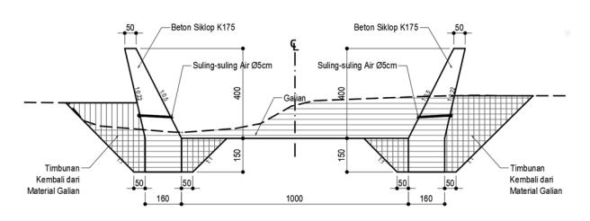
Figure 1. the river's cross section after construction. (Source: River Basin Management of Sulawesi III)
4. Research Method
In order to obtain the necessary information for numerical modelling, topographical data such as Digital Elevation Model (DEM), land cover and Harmonized World Soil Database (HWSD) maps were collected. Furthermore, hydrological data such as rainfall data was collected from 3 (three) rain gauge stations for the duration of 19 (nineteen) years. The topographical and hydrological data were analysed to obtain the river's hydrograph according to the appropriate procedure (SNI-241, 2016). Field data such as instantaneous discharge, bed material, and suspended solid concentration was also collected according to the appropriate standard and procedure (SNI-8066, 2015; SNI-3414, 2008).
A numerical model for hydraulic and sediment transport analysis uses hydrograph as the upper boundary, while coupled sediment modelling gives a more complete picture of morphological changes (Garegnani, et, al., 2011), HEC-RAS sediment transport modelling proved to be robust enough for modelling river (Joshi, 2019) and high sediment concentration flow such as dam flushing (Gibson, at., 2019), therefore due to the concentration of normal river such as Paneki River is far from dam flushing event (Gibson, at., 2019) HEC-RAS is used for modelling Paneki River. River geometry data is obtained from shop drawings, and the field data that was collected is used to model the river bed gradation and both theoretical and field sediment rating curve (Yang, 1996).
River discharge capacity is obtained by subjecting the river model to a number of hydrographs. The result is then further analysed to gain the maximum discharge at which the river is on the brink of overflowing. The bed morphological changes of the model are obtained by conducting sediment transport analysis of the model with the corresponding boundary for sediment transport analysis and discharge hydrographs as the upper boundary and not by satellite imagery for river's lateral morphological changes (Kurniawan, at al., 2017).
5. Result
5.1 Topographic analysis
Using GIS-based software, the area of the watershed could be delineated. Furthermore, the coefficient for Thiessen rainfall area and the curve number of said watershed could also be obtained for rainfall area calculation and rainfall abstraction, respectively. It is obtained that the area of the watershed is 60.42 km2 , with a curve number of 63.14. Also, the coefficient for the Thiessen rainfall area method is presented in the following table:
Table 1. Thiessen coefficient for Paneki watershed
| Station | Polygon Area [km2 ] | Thiessen Coefficient |
|---|---|---|
| Porame | 0.98 | 0.02 |
| BMKG | 9.48 | 0.16 |
| Bora | 49.96 | 0.83 |
| Sum | 60.42 | 1.00 |
5.2 Hydrologic analysis
Using rainfall data from three stations near the watershed and the result from topographical analysis, hydrologic analysis using Synthetic Unit Hydrograph (SUH) was performed due to the lack of discharge data in the river and in accordance with the procedure for flood discharge calculation (Gibson, at., 2019), the necessary hydrograph for various return periods
needed for hydraulic and sediment transport model analysis could be obtained.
5.3 Calibration of hydrologic and hydraulic models
A bankfull discharge approach was taken in order to calibrate the hydrologic model in an ungauged watershed such as the Paneki River. Manning's roughness coefficient is obtained from multiple instantaneous discharge measurements at the inlet of the field where the river is still in its natural state. Using the cross-sectional data and calculating the inflection point of discharge against the depth relationship (Parker, 2004) the bankfull depth is determined at 0.67 m. Assuming the flow is steady, the bankfull discharge could be calculated as follows:
\[Q = \frac{1}{n}R^{2/3}S^{1/2}A = \frac{1}{0.037} \left(\frac{5.05}{12.53}\right)^{2/3} (0.0082)^{1/2} = 6.81 \text{ m}^3\text{s}^{-1}\]
The return period of bankfull discharge is around 2.33 years (Dalrymple, 1960) and within the range of 1 - 5 years in the flood frequency analysis (Julien, 2018). In this study, it is assumed that the bankfull discharge return period is 2 years. Therefore, the SUH could be calibrated using the bankfull discharge obtained above. The calibrated hydrograph for the downstream Paneki River is as follows:
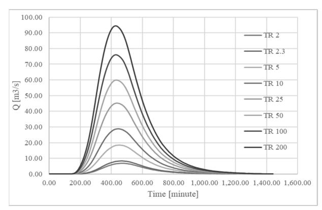
Figure 2. Calibrated hydrograph for downstream Paneki river
The hydraulic analysis of the model was conducted using field measurements of instantaneous discharge on the downstream Paneki River. From the field measurement, it was obtained that the discharge was 3.056 m³/s. The water depth was 0.258 m. By changing the Manning's coefficient of the model, we could simulate similar conditions in the model in which at a discharge of 3.056 m³/s the water depth at the measurement area is 0.258 m, and changing the Manning's roughness of the hydraulic model by trial and error, it was found that at a Manning's coefficient of 0.0225, the depth of the numerical model approaches that of the measured on the field.
5.4 Hydraulic model analysis
Simulation for flood events uses hydrograph data hydrologic analysis. The upstream boundary uses a flow hydrograph for each planned return period to simulate flood events in the Paneki River. This discharge with a return period is taken in accordance with the Palu River
flood disaster mitigation plan, which uses a discharge with a return period of 25 years, while for other periods it is used to obtain the capacity of the river to flow discharge where the water depth is at full depth. The result from the hydraulic model is as follows:
Table 2. Hydraulic model result
| No | Q [m3/s) | h [m] | Clearance [m] |
|---|---|---|---|
| 1 | 45.30 | 1.39 | 2.61 |
| 2 | 59.80 | 1.62 | 2.38 |
| 3 | 76.10 | 1.88 | 2.12 |
| 4 | 94.32 | 2.15 | 1.85 |
| 5 | 121.56 | 2.52 | 1.48 |
| 6 | 144.70 | 2.81 | 1.19 |
From the table above, we could surmise that even at 144.70 m<sup>3</sup>/s, the river is still not full. Therefore, from the result above, the relationship between depth and discharge is obtained to find the maximum capacity of the river.
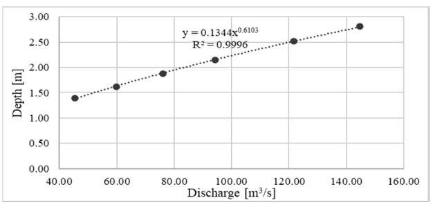
Figure 3. Graph of relationship between discharge and depth for downstream Paneki river.
From the relationship depicted in the graph above, we could calculate the discharge of the river at a maximum depth of 4 m, as follows:
\[h = 0.1344 Q^{0.6103}\] \[Q = \left(\frac{h}{0.1344}\right)^{1/0.6103} \rightarrow Q = \left(\frac{4}{0.1344}\right)^{1/0.6103} = 259.81 \text{ m}^3 \text{s}^{-1}\]
Therefore, at a discharge of 259.81 m<sup>3</sup>/s, the Paneki River is at its maximum capacity at a water depth of 4 m.
5.5 Sediment transport model analysis
The sediment transport analysis is to be carried out for several scenarios to get a pattern of morphological changes in the river to transport function, changes in the river bed to multiple discharge events, and the effect of a consolidation dam (CD) in the river. The general scheme for the sediment transport model analysis is as follows Figure 4.
In order to achieve the goal of the sediment transport simulation, multiple simulation scenarios are conducted as follows: Simulation 1: This simulation is carried out using Q2 discharge and three transport functions, namely: Yang, Ackers and White, and Tofaletti—eyer Peter Müller (MPM) to get the difference between each equation on changes in the morphology of the model
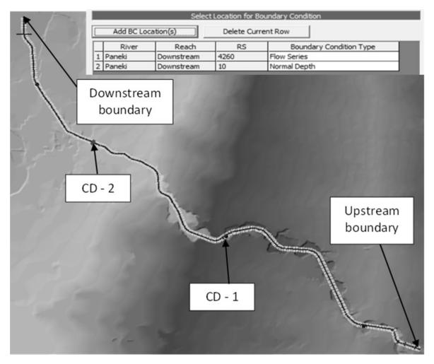
Figure 4. Sediment transport analysis modelling scheme
river. Simulation 2: This simulation uses daily discharge for 1 year to see the model's response to multiple events. The simulation also uses a transport function selected from the results of simulation 1. Simulation 3: This simulation changes the location of CD-2 to get the effect of CD-2 on river morphology, with daily discharge for 1 year with Q2 as the inflow boundary, and using the transport function selected from the previous simulation.
To carry out a study on changes in river morphology in the form of aggradation and degradation of the riverbed, the Paneki River is divided into 3 (three) parts, namely: the downstream part, which is the area from the river outlet to CD-2, the middle part, which is between CD-2 and CD-1, and the upstream part, which is the area from CD-1 to the river inlet. The results that will be reviewed from the model are changes in river bed elevation, or aggradation and degradation as a form of changes in the morphology of the Paneki River to the flow in the field, or Q2.
5.5.1 Simulation 1
This simulation was carried out using the same river geometry as hydraulic analysis, with a Q2 discharge for 1 (one) year, using 3 (three) transport functions, namely the Yang, Ackers-White (AW), and Meyer-Peter-Müller-Toffaleti (MPM-TF) equations.
From the graph above, it can be seen that in the upstream area (before CD-1) the three methods provide simulation results in the form of river degradation, where the Acker-White (AW) method gives fairly
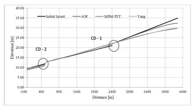
Figure 5. Simulation – 1 invert elevation result.
good modeling results, while the other two methods give quite large degradation results. It could also be seen that the AW and Yang methods gave a relatively similar bed change pattern, while the results using the MPM-TF transport function gave quite different results, especially in the middle and downstream areas. The summary of the analysis is presented in the following Table 3.
From the table above, it can be seen that the pattern of aggradation and degradation in river morphology using the Ackers – White and Yang equations have relatively the same results for all parts of the river, where degradation occurs in the downstream area of the river, and in the middle area tends to be stable which is dominated by river aggradation, while the upstream area degradation occur. Hence, for simulation 2 and 3 Ackers – White transport function will be used for sediment transport analysis.
5.5.2 Simulation 2
This simulation was carried out using a 1 (one) year discharge generated from the 2019 rainfall data. The sediment transport functions used are Ackers and White from the simulation-1 result, and the geometry used is the same as in simulation-1.
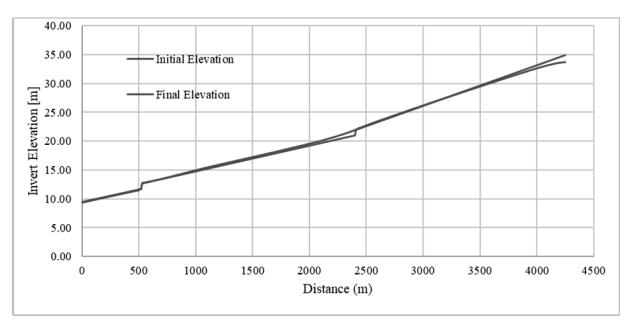
Figure 6. Simulation - 2 invert elevation result
Table 3. Sediment transport simulation - 1 result summary
| Yang | Ackers - White | MPM - Toffaleti | |||||||
|---|---|---|---|---|---|---|---|---|---|
| Region | Max Aggradation (m) | Max Degradation (m) | Average D invert (m) | Max Aggradation (m) | Max Degradation (m) | Average D invert (m) | Max Aggradation (m) | Max Degradation (m) | Average D invert (m) |
| Downstream | 0.02 | -0.92 | -0.80 | 0.01 | -0.57 | -0.47 | 0.37 | 0.00 | 0.20 |
| Middle-stream | 0.02 | -0.92 | -0.80 | 0.01 | -0.57 | -0.47 | 0.37 | 0.00 | 0.20 |
| Upstream | 0.12 | -5.00 | -2.03 | 0.08 | -2.50 | -0.60 | 1.66 | -1.07 | 0.06 |
From the graph above, it can be seen the changes in the morphology of the Paneki River model. From the simulation results, it is found that the downstream area is degraded, the middle area is aggraded, and in the upstream area there is degradation near the river inlet and aggradation in the vicinity of CD-1. The summary of the simulation–2 sediment transport analysis is presented in the following Table 4.
In the downstream part, degradation occurs. The average degradation that occurs in the upstream area over one year is 0.12 m, while the highest aggradation that occurred was 0.02 m, and the highest degradation that occurred in this area was 0.17 m in the 9th month. In the middle section of the average model of river morphology, changes occur in aggradation overall. The average morphological change that occurs in this area at the end of the simulation is an aggradation of 0.27 m, with a maximum aggradation that occurs in this area of 0.90 m. In the upstream part, it can be seen that in this area, degradation tends to occur with an average degradation of 0.17 m until the end of the one-year simulation. The maximum degradation that occurs in this area is 1.24 m. The aggradation that occurs in this area is quite small where the location of the aggradation occurs around CD-1.
5.5.3 Simulation 3
This simulation uses a bank full discharge with a simulation duration of 1 year. The transport function used is Ackers–White. The geometry used in this simulation varies where the position of CD–1 is fixed while the position of CD–2 varies relative to the downstream of the model with the following configuration: 1. at 340 m, 2. at 440 m, 3. at 540 m, 4. at 640 m, and 5. at 740 m.
The graph above shows the elevation and longitudinal cumulative mass change of the river model changing in response to the location of CD – 2, which from the elevation graph can be seen that in the upstream area of CD – 1, degradation occurs, then the river bed becomes stable in the area near CD – 1, in the middle area there is aggradation, and finally in the downstream area, degradation occurs for all positions of CD – 2.
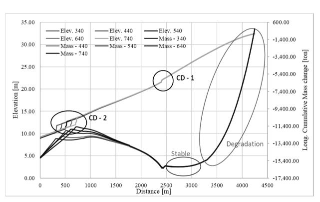
Figure 7. Simulation - 3 invert elevation and longitudinal cumulative mass change
It can be seen from the cumulative longitudinal mass graph that the influence of variations in the position of CD–2 on sediment mass transfer in the middle area decreases until it is relatively no longer influential at a distance of 2000 m. Furthermore, the influence of position variance of CD–2 can no longer be seen to have an effect on changes in river morphology in the upstream area.
From the model simulation results, it is found that the downstream area is the area most affected by variations in the position of CD-2. It can be seen from the table above that the farther the position of CD-2 from the downstream, the greater the degradation that occurs in this area, where a maximum degradation of 1.46 m occurs on the CD-2 configuration at a position of 740 m from the downstream. From the average change in the
Table 5. Morphological changes in downstream part of the river (Simulation - 3)
| CD - 2 Position [m] | Max degradation [m] Average ÿ Invert [m] | |
|---|---|---|
| 340 | -0.62 | -0.51 |
| 440 | -1.46 | -0.66 |
| 540 | -1.48 | -0.80 |
| 640 | -1.34 | -0.74 |
| 740 | -1.46 | -0.91 |
Table 4. Sediment transport analysis simulation - 2 result summary
| No | Parameter | Downstream | Middle | Upstream |
|---|---|---|---|---|
| 1 | Max Aggradation invert -3mo (m) | 0.01 | 0.08 | 0.05 |
| 2 | Max Degradation invert -3mo (m) | -0.06 | -0.04 | -0.28 |
| 3 | Average D invert 3mo (m) | -0.01 | 0.01 | -0.02 |
| 4 | Max Aggradation invert -6mo (m) | 0.01 | 0.59 | 0.08 |
| 5 | Max Degradation invert -6mo (m) | -0.15 | -0.02 | -1.21 |
| 6 | Average D invert 6mo (m) | -0.09 | 0.12 | -0.16 |
| 7 | Max Aggradation invert -9mo (m) | 0.01 | 0.62 | 0.20 |
| 8 | Max Degradation invert -9mo (m) | -0.17 | -0.03 | -1.24 |
| 9 | Average D invert 9mo (m) | -0.12 | 0.14 | -0.20 |
| 10 | Max Aggradation invert -12mo (m) | 0.02 | 0.90 | 0.15 |
| 11 | Max Degradation invert -12mo (m) | -0.14 | 0.00 | -1.24 |
| 12 | Average D invert 12mo (m) | -0.12 | 0.27 | -0.17 |
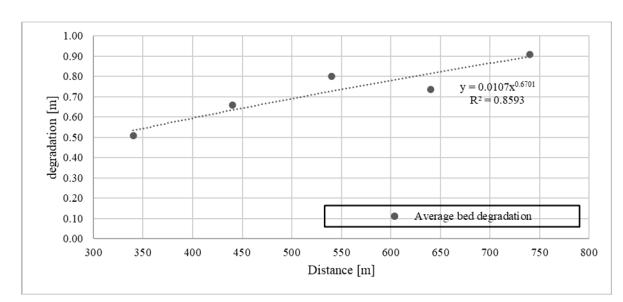
Figure 8. Relationship between average degradation and variation of CD - 2 positions.
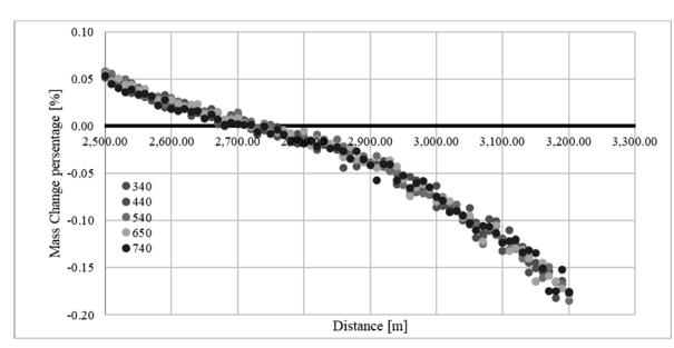
Figure 9. Influence of variation of CD - 2 position to invert stabilization in upstream part.
riverbed in the table above, it is also greater if the position of CD-2 is further downstream. For the minimum downstream river degradation, the most optimal configuration is the position of CD-2 at a distance of 340 m from the downstream.
Using the graph above, we can obtain an equation that relates the average degradation in the downstream area to the position of CD-2, namely: y=0.0107x 0.6701; where y is the average depth of degradation [m] and x is the relative CD-2 position from the downstream [m].
The graph above shows the effect of CD-1 (2410 m) on stabilizing degradation in the river model, where at a distance of 2740 m, the presence of CD-1 is able to stabilize mass changes in this area and further assure the effect of variance in the position of CD-2 is negligible in the upstream part of the model.
The relationship between the percentage change in mass and the distance in the middle area can be seen on the graph above, where it should also be noted that the presence of CD-1 in the upstream will affect the ability of CD-2 to stabilize the river. It is assumed that the quadratic equation represents the relationship between each CD-2 configuration and mass transfer. From this, it can be obtained the distance where the river morphology in the middle area is stabilized by CD-2. By differentiating the equations above, we can get the points of maxima for each CD-2 position variation. Each point then can be seen on the graph below (Figure 11).
Using the equation from the graph above, the optimum distance for the position of CD-2 can be obtained as follows:
\[y = -1018 \ln(x) + 7208.1 \rightarrow \ln(x) = \frac{7208 - y}{1018} \rightarrow x = e^{7208 - y} / 1018\]
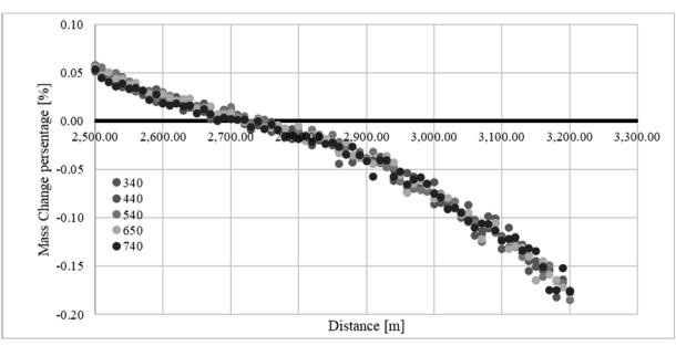
Figure 10. Relationship between long. Mass cumulative change and variation of CD - 2 position
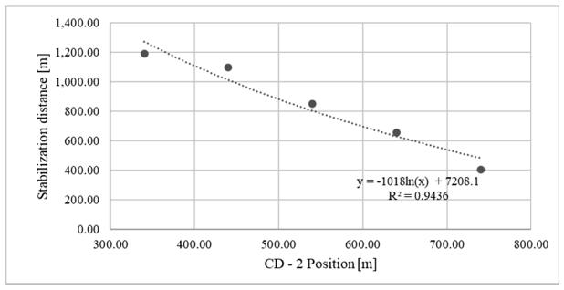
Figure 11. Stabilization distance due to variation of CD - 2 positions.
Solving for y = x, then x = 636.27 m
6. Conclusion
From this study we could conclude that:
- 1. The height of the built river bank is sufficient to accommodate a discharge of 259.81 m3 /s for clear water condition, and the designed cross-section is to accommodate mudflow discharge just like the condition post disaster in 2018;
- 2. The results of Simulation-1 show that the Ackers-White and Yang methods give similar results compared to the MPM-Toffaleti method;
- 3. The results of simulation 2 of the model show that there is aggradation and degradation in the upstream part of this river where from the model results obtained a maximum aggradation of 0.15 m and a maximum degradation of 1.24 m;
- 4. The middle part is relatively stable in general, but it is necessary to pay attention to the aggradation that occurs in the upstream area of CD – 2;
- 5. At the downstream area of the river there is river degradation, where the average degradation from the model results in this area is 0.12 m, with a maximum degradation of 0.14 m;
- 6. The results of river model for simulation 3 show the effect of the CD-1 consolidation dam for bed stabilization were up to the distance of 2740 m relative to the river's outlet;
- 7. At the middle part of this river model, the stabilization effect of CD – 2 on this area is described by the equation y = -1018 ln(x) +7208.1; and
Acknowledgments
Authors wishes to acknowledge assistance and encouragement from graduate advisors Mr. Dhemi Harlan and Mr. Arie Setiadi Moerwanto, colleagues, staff of Water Resources Engineering and Management Program and finally to Ministry of Public Works and Housing for its financial support.
References
- Dalrymple. T (1960). Flood Frequency Analyses; Manual of Hydrology: Part 3. Flood-Flow Techniques, Geological Survey Water-Supply Paper. Washington
- Garegnani, G. et al. (2011). Free Surface Flows Over Mobile Bed: Mathematical Analysis and Numerical Modeling of Coupled and Decoupled Approaches. Communications in Applied and Industrial Mathematics, 371.
- Gibson, S. et al. (2019). Modeling Sediment Concentrations During a Drawdown Reservoir Flush: Simulating the Fall Creek Operations with HEC-RAS. Engineering Research & Development Centre, USACE.
- Gibson, S. et al. (2019). Modeling Sediment Concentrations During a Drawdown Reservoir Flush: Simulating the Fall Creek Operations with HEC-RAS. Engineering Research & Development Centre, USACE.
- Gibson. S, et al (2020). HEC-RAS: Sediment Transport User's Manual Version 6.0, US Army Corps of Engineers, California.
- JICA (2019). Detailed Design on Additional Servis After The 2018 Earthquake at Central Sulawesi – Sub Project No. B9: Downstream of Paneki River.
- JICA (2019). Reconstruction Project for Central Sulawesi for Sediment Disaster – Project Summary.
- Joshi, N. et al. (2019). Application of HEC-RAS to Study Sediment Transport Characteristic of Maumee River in Ohio.
- Julien, P. Y (2018). River Mechanics 2nd Edition, New York: Cambridge University Press.
- Kurniawan, R. et al. (2017). Analisis Perubahan Morfologi Sungai Rokan Berbasis Sistem Informasi Geografis dan Penginderaan Jauh.
- National Standard Agency, (2008). SNI 3414:2008 Tata Cara Pengambilan Contoh Muatan Sedimen Melayang di Sungai dengan Cara Integrasi Kedalaman Berdasarkan Pembagian Debit, Jakarta.
- National Standard Agency, (2015). SNI 8066:2015 Tata Cara Pengukuran Debit Aliran Sungai dan Saluran Terbuka Menggunakan Alat Ukur Arus dan Pelampung, Jakarta.
- National Standard Agency (2016). SNI-2415-2016 Tata Cara Perhitungan Debit Banjir Rencana, Jakarta.
- Parker, G (2004). 1D Sediment Transport Morphodynamics with Applications to Rivers and Turbidity Currents.
- Yang, C. T (1996). Sediment Transport: Theory and Practices, New York: McGraw-Hill.
River Morphological Study of Downstream Paneki...