
Abstrak
Studi ini mengusulkan prosedur baru terkait penyesuaian spektra catatan percepatan gempa. Prosedur ini dilakukan dengan mempertahankan sudut phasa tetapi mengubah amplitudo Fourier catatan percepatan gempa demikian hingga spektrumnya sesuai dengan target. Target spektrum yang diinputkan mewakili tiga komponen gempa. Untuk mengujinya, beberapa catatan gempa tiga-komponen disesuaikan spektrumnya terhadap dua target spektra. Ketelitian yang cukup baik terlihat dari catatan kecepatan dan simpangan. Skala ketiga komponen juga dijaga sehingga dihasilkan percepatan gempa tiga-komponen yang realistis. Percepatan gempa sejenis ini diperlukan dalam proses kualifikasi struktur penting yang sensitif terhadap pengaruh gerakan tiga arah. Prosedur tersebut adalah baru karena teknik yang ada sekarang didasarkan pada penyesuain spektrum per-komponen.
Kata-kata Kunci: Penyesuaian spektra, tiga komponen, skala komponen, sudut phasa, struktur penting.
1. Introduction
The need for realistic ground motions is the most critical issue in seismic analyses and design of critical structures. Recorded (three-component) earthquake motions are preferred to produce a realistic structural response (ASCE/SEI, 2019). However, the appropriate ground motion records of earthquakes for a particular site are rarely available (Wang et. al., 2014). In such cases, a suite of derived records must be generated via synthetic procedures or through spectral matching of recorded records or seeds. While some parameters are maintained (e.g., the scales1 among the three components), the others such as Fourier amplitudes and phases, durations, and peaks as well as spectral amplitudes are altered following the spectral
adjustments. This study proposes a novel, yet simple, procedure to generate spectrum-compatible threecomponent seismic ground accelerations based on the seed records to be used in the response analyses of critical structures. These cases are not only limited to nuclear structures as specified in ASCE/SEI (2019) but also extendable to include tall building structures, large dams, and long-span bridges. Unlike the present spectral matching practices that process the three components based on individual component separately, in this study, we performed spectral matching on three components simultaneously and treated it as a vector.
Aside from three-component procedure, onecomponent spectral matching has long history. One good literature review could be found in Li et. al.
1The scales are the ratios among the components' magnitudes.
(2017). The matching processes could be performed either in frequency domain (Rizzo et. al., 1975, Gasparini and Vanmarcke, 1976, Kost et. al.,1978, Preumont, 1984, Bani-Hani and Malkawi, 2017), time domain (Kaul, 1978, Lilhanand and Tseng, 1988, Abrahamson, 1992, Mukherjee and Gupta, 2002, Suárez and Montejo, 2005, Hancock et. al., 2006, Al Atik and Abrahamson, 2010, Ni et. al., 2011, Gao et. al., 2014, Adekristi and Eatherton, 2016, Li et. al., 2016), or both (Preumont, 1984, Silva and Lee, 1987). In frequency domain spectral matching, the Fourier amplitude and phase spectra are iteratively adjusted until the acceleration spectral ordinates agree with that of the target. In time domain, the acceleration time series are iteratively modified until agreement of the acceleration response spectrum to that of target are achieved. The modification could be done by adding series of wavelets (Kaul, 1978, Lilhanand and Tseng, 1988, Abrahamson, 1992, Mukherjee and Gupta, 2002, Suárez and Montejo, 2005, Hancock et. al., 2006, Al Atik and Abrahamson, 2010, Gao et. al., 2014, Adekristi and Eatherton, 2016) or by decomposing the original record into mode functions, adjusting, and then recombining them (Ni et. al., 2011, Li et. al., 2016). A technique employing an eigenfunction expansion of the seeds has also been proposed (Li et. al., 2017). Most of these works were applied to onecomponent acceleration records, except Ni et. al. (2011), Li et. al. (2016) and Yang et. al. (2021) who tried extending the technique to three-component records, apparently after realizing that using threecomponent ground motions is necessary in structural analyses that are sensitive to three-component motions, likely arising from the stiffness and/or mass irregularities existing in structures. This is emphasized in Section 3.1 of ASCE/SEI (2019) that requires seismic demand to be obtained for three translational earthquake motions.
Ni et. al. (2011) proposed that three-component matching be carried out sequentially for two horizontal components and separately for vertical direction. The procedure started with first-horizontal-component spectral matching against a horizontal target spectrum. This step is followed with the second-horizontalcomponent based on the first component in such a way that condition on statistical independence of both components is satisfied. The second component satisfies the same horizontal target spectrum as the first. Lastly, the vertical component is matched based on the actual vertical acceleration record until its response spectrum agree with vertical target spectrum. This process is performed by Hilbet-Huang transformation (HHT) allowing modifications of both the amplitude and phase of the actual records as function of time. In this technique, there are two different target spectra needed, for horizontal and vertical components. Li et. al. (2016) performed the procedure to three components independently with its own target spectrum using HHT keeping the statistical independence of the three. Similarly, Yang et. al. (2021) basically using the method of Li et. al. (2017) combined with other technique to produce fully independent three-component matched records; however, the procedure was performed individually for different horizontal dan vertical target spectra. These very complex operations would change the functional relation among the components or the direction cosines of the earthquake acceleration vector to the degree that the resulting waveform might be entirely different from its recorded counterpart and might not be an earthquake waveform anymore, which is to be avoided in this study.
The above discussion suggests the necessity of maintaining the direction cosines of the acceleration vector during spectral matching. Not only does it important to maintain the direction cosines but also not to disturb too much the Fourier spectrum is necessary if the property of the actual waveform is to be managed (Carlson et. al., 2016). This is true for the Fourier phase because some studies showed that there is structure or pattern in phase spectrum. These studies found that the distribution of the Fourier phase tended to be uniform, and the distribution of the difference of any two consecutive phases appeared to be normal. Furthermore, the waveform of the actual records and their phases were very similar (Ohsaki, 1979). The phase distribution also might have an important impact on the inelastic structural response (Tiliouine et. al., 2000). Therefore, accurately reproducing the real phase in the simulated records is crucial (Thrainsson et. al., 2000). In other investigations, replacing the phase record with that of others yielded modified records of the same peak ground acceleration (PGA) but entirely different nonlinear SDOF responses (Tao et. al., 2019). Moreover, we found that the phases of seismic records form spiral patterns (see Section 3); therefore, maintaining the phases is important ASCE/SEI (2019). This suggests that the only freedom rests with the adjustments of the Fourier amplitude spectrum (FAS). For this purpose, the most straightforward technique is the eigenfunction expansion of the actual records, which allows controlling the amplitude and phase spectra independently. The simplest form of this technique is the Fourier transform method and will be used in the following development.
In Fourier transform method, the seed time series is Fourier transformed to obtain the corresponding frequency series, expressed as the product of Fourier amplitude and phase spectra. Both the amplitude and phase can be modified by using a frequency-dependent filter function \(P(\omega) = |P(\omega)|e^{i\phi P(\omega)}\), where \(|P(\omega)|\) and \(\phi\) \(P(\omega)\) are the filter's amplitude and phase, respectively. The modification is performed iteratively until the response spectrum of the resulting time series agree with a given target. In this study a single target spectrum is used, and it should incorporate both the horizontal and vertical components. The seed's Fourier amplitude spectrum (FAS) is also incorporating its three components. It is preferable that the target spectrum
The direction cosine of vector a is defined as \(\ell_i = a_i/|\mathbf{a}|\) for its \(i^{\text{th}}\)-component (i=1,2,3), where \(|\mathbf{a}| = \sqrt{\sum_i a_i^2}\) is its magnitude; consequently \(\sum_i \ell_i^2 = 1\)
is in the form of the pseudo-velocity spectrum \((S_{p\nu})\) as there is 'similarity' between \(S_{pv}\) and FAS.
The spectral matching using a scalar filter function that operates on a vector of three components would maintain the ratio among the components and thus their direction cosines; otherwise, a spectral scaling could be carried out to the vertical component. Both the filter's amplitude and phase could be adjusted but adjusting the phase would not change the phase difference among the components, while adjustments of the filter's amplitude are operated on the modified record's FAS until agreement on the modified record's spectrum to that of a target was achieved. The simplest procedure, known as spectral scaling, involves fixing the amplitude, \(|P(\omega)| = \text{constant}\), and setting the filter's phase to be identically zero, \(\phi P(\omega) = 0\), and resulting in the modified record having a phase identical to the seed and a Fourier amplitude spectrum proportional to that of the seed record.
In this study, the seeds were retrieved from the Pacific Earthquake Engineering Research Center (PEER, 2022) (or other agencies) by focusing to those with their spectra close to the target (assumed to be given). This closeness is necessary so that the modified records are not too much distorted from the seeds (Wang, et. al., 2014, Kohrangi et. al., 2017, Baker and Lee, 2018, ASCE/SEI, 2019). The average spectrum of all seeds was be produced and compared to that of the target. In this study, this average spectrum was used as an alternative to the target.
The development starts by considering a mass excited in three orthogonal directions by three-component ground acceleration. The motion in each direction is associated with distinct component, and its dynamical properties, spring, and damping are identical in all directions (i.e., isotropic) and constant. The methodology and problem formulation are discussed in next section.
2. Methodology and Problem Formulation
Consider a mass excited by three-component ground motion with a linear spring and damping system. The equation of motion of the mass can be expressed as follow (Clough and Penzien, 2003, Chopra, 2020)
\[\mathbf{M} \frac{d^2}{dt^2} \mathbf{u}(t) + \mathbf{C} \frac{d}{dt} \mathbf{u}(t) + \mathbf{K} \mathbf{u}(t) = -\mathbf{M} \mathbf{a}(t)\] (1)
where M, C, and K are the 3 x 3 mass, damping, and stiffness matrices, respectively (assumed to be constants), \(\mathbf{u}(t)\) is the three-component displacement vector of the mass, and \(\mathbf{a}(t)\) is the three-component translational ground acceleration vector. For an isotropic system excited by the seed ground acceleration, Eq. (1)
\[\frac{d^2}{dt^2}\boldsymbol{u}_s(t) + 2\zeta\omega_n \frac{d}{dt}\boldsymbol{u}_s(t) + \omega_n^2 \boldsymbol{u}_s(t) = -\boldsymbol{a}_s(t) \quad (2)\]
Where \(\mathbf{a}_{s}(t) = (\mathbf{a}_{s1}(t), \mathbf{a}_{s2}(t), \mathbf{a}_{s3}(t))\) (\(\mathbf{u}_{s}(t)\) can be expressed similarly), \(\zeta\) is the damping, and \(w_n\) is the system's natural frequency (\(\zeta\) and \(\omega_n\) are constants). While the notation \(\mathbf{u}_{s}(t)\) is employed in the time domain, the notation \(u_s(\omega)\) is employed in frequency domain for its
transformed quantity. The solution to Eq. (2) for the displacement in frequency domain is
\[\mathbf{U}_{s}(\omega) = -H(\omega; \omega_{n}, \zeta) \mathbf{A}_{s}(\omega)\] (3)
where \(U_s(\omega) = \int_{-\infty}^{\infty} u_s(t) e^{-i\omega t} dt\) is the Fourier transform of \(\mathbf{u}_{\mathrm{s}}(t), H(\omega; \omega_n, \zeta) = |H(\omega; \omega_n, \zeta)| \ e^{i\varphi_H(\omega; \omega_n, \zeta)}\)
is the frequency response function in which
\[|H(\omega;\omega_n,\zeta)| = \frac{1}{{\omega_n}^2} \sqrt{\frac{1}{[1-(\omega/\omega_n)^2]^2 + [2\zeta\omega/\omega_n]^2}} \text{ and}\]
\[\tan \varphi_H(\omega; \omega_n, \zeta) = \frac{2\zeta\omega/\omega_n}{1 - (\omega/\omega_n)^2}\], and
\[A_s(\omega) = \int_{-\infty}^{\infty} a_s(t) e^{-i\omega t} dt\] is the Fourier transform of the seed ground acceleration vector (the details could be found in Clough and Penzien, 2003). The right side of Eq. (3) contains two kinds of phases: the first is the phase between the motion and the response embedded in the response function, and the second is the built-in Fourier phase in the ground acceleration.
The Fourier amplitude spectrum (FAS) of u<sub>s</sub> is defined as \(FAS_{u_s}^2(\omega) = U_s(\omega) \cdot U_s(\omega) *\), where the symbol • represents the inner product and * represents the conjugate. Using Eq. (3), the FAS can be obtained through the expression
\[FAS_{\mathbf{u}_s}(\omega) = |H(\omega; \omega_n, \zeta)| \quad FAS_{\mathbf{a}_s}(\omega) \tag{4}\]
Similarly, the Fourier amplitude spectrum of the modified record, \(U_m(\omega)\), can be obtained as
\[FAS_{\mathbf{u}_m}(\omega) = |H(\omega; \omega_n, \zeta)| \quad FAS_{\mathbf{a}_m}(\omega)\] (5)
Let a filter function \(P(\omega)\) be the ratio of Eq. (5) to Eq. (4). Then the following two equations hold:
\[FAS_{\mathbf{u}_m}(\omega) = |P(\omega)| \ FAS_{\mathbf{u}_s}(\omega) \tag{6}\]
\[FAS_{a_m}(\omega) = |P(\omega)| \ FAS_{a_s}(\omega) \tag{7}\]
Eq. (7) shows that the filter function \(P(\omega) = |P(\omega)|e^{i\phi P(\omega)}\), where \(|P(\omega)|\) and \(\phi P(\omega)\) are the filter's amplitude and phase, respectively, completely controlling the modification of the seed acceleration into the modified acceleration. Eq. (6) indicates that the adjustments of the responses are completely described by the same function. Further operations on Eq. (7) leads to
\[A_m(\omega) = P(\omega) A_s(\omega) \tag{8}\] where the indices m and s represent the modified and seed ground accelerations, respectively. Because A(-ω) = \([\mathbf{A}(\omega)]\)* for real \(\mathbf{a}(t)\), it follows that \(P(-\omega)=[P(\omega)]\)* or \(\phi_P(-\omega) = -\phi_P(\omega)\) (Press et. al., 2007), where * denotes conjugation.
If \(P(\omega)\) is obtained as the Fourier spectral ratio, as indicated by Eq. (7), then Eq. (8) is exact. However, when \(P(\omega)\) is determined by the response spectral ratio (instead of the Fourier spectral ratio), Eq. (8) is merely an approximation. There is a similar relation for the Fourier and pseudo-velocity spectra, expressible as (for low damping; \(\zeta \leq 0.10\)) (Hudson, 1962)
\[FAS_a(\omega) = \sqrt{\sum_{i=1}^{3} \left\{ \left( \int_0^{t_D} a_i(\tau) \operatorname{sin}\omega \tau d\tau \right)^2 + \left( \int_0^{t_D} a_i(\tau) \cos \omega \tau d\tau \right)^2 \right\}}\](9)
\[S_{pv}(\omega) \le \max_{t} \sqrt{\sum_{i=1}^{3} \left\{ \left( \int_{0}^{t} a_{i}(\tau) \sin \omega \tau \ d\tau \right)^{2} + \left( \int_{0}^{t} a_{i}(\tau) \cos \omega \tau \ d\tau \right)^{2} \right\}}\](10)
where \(FAS_{\mathbf{a}}(\omega)\) is the Fourier amplitude, \(S_{pv}(\omega)\) is the pseudo-velocity spectra, and \(t_D\) is the duration of the record. When Eq. (9) is used for the spectral ratio to obtain \(|P(\omega)|\) in Eq. (8), then the modified ground acceleration can be computed in a straightforward manner. However, when Eq. (10) is employed to compute \(|P(\omega)|\), then Eq. (8) is only an approximation, and iteration is necessary to solve the matching process.
The inverse transform of Eq. (8) is
\[a_m(t) = \frac{1}{2\pi} \int_{-\infty}^{\infty} \int_{-\infty}^{\infty} a_s(\xi) \ e^{-i\omega\xi} \ d\xi \ P(\omega) \ e^{i\omega t} \ d\omega \quad (11)\]
Interchanging the order of integration and recognizing that, \[p(t) = \frac{1}{2\pi} \int_{-\infty}^{\infty} P(\omega) e^{i\omega t} d\omega\] one can obtain the convolution integral
\[a_m(t) = \int_0^{t_D} a_s(\xi) \ p(t - \xi) \ d\xi \tag{12}\] where p(t) is real because \(P(-\omega)=[P(\omega)]*\), and \(t_D\) is the length of the time series.
Eq. (12) forms the basis to obtain the modified ground acceleration when given seed records, with p(t) expresses the ratio of the seed and the target spectra. It is now necessary to investigate whether the ratios of the components of the seed's acceleration are preserved by the modified record following the operation by Eq. (12). These ratios are related to their direction cosines both in time and frequency domains. Let \(L_{amj}(\omega)\) be the \(j^{th}\)-component direction cosine of a complex-valued vector \(\mathbf{A}_m(\omega)\), and \(l_{amj}(t)\) be the \(j^{th}\)-component direction cosine of a real-valued vector \(\mathbf{a}_m(t)\), which are expressed as
\[L_{amj}(\omega) = \frac{A_{mj}(\omega)}{|A_m(\omega)|} = \frac{|P(\omega)| \ e^{i\varphi_P(\omega)} A_{sj}(\omega)}{|P(\omega)||A_s(\omega)|} = e^{i\varphi_P(\omega)} \ L_{asj}(\omega)\](13)
\[l_{amj}(t) = \frac{a_{mj}(t)}{|a_m(t)|}\] (14)
Eq. (13) shows that the amplitudes of \(L_{amj}(\omega)\) are always preserved because \(|L_{amj}(\omega)|=|L_{asj}(\omega)\) for the modified and seed records (j=1,2,3). However, comparing Eqs. (13) and (14), \(L_{amj}(\omega)\) and \(l_{amj}(t)\) would not form a Fourier transform pair because the amplitudes \(|\mathbf{A}_m(\omega)|\) and \(|\mathbf{a}_m(t)|\) are not paired. Consequently, the direction cosines of the time series cannot be preserved at any time t, or \(l_{amj}(t) \neq l_{asj}(t)\). This is also observed in Eq. (12) as its ratios or the direction cosines of the components' time series are preserved only when p(t) is proportional to a Dirac delta function, which is the case of uniform spectral scaling of all components; otherwise, they would not be preserved. The latter corresponds to a constant \(P(\omega)\), producing modified records which are proportional to the seeds.
Although the time series direction cosines cannot be preserved at any time t, they can be maintained in an average sense by adjusting the frequency series directions cosines, \(L_{amj}(\omega)\) (j=1,2,3). As will be discussed later, it would be necessary to modify the frequency direction cosines of the vertical component in some cases. Consequently, the direction cosines of the other components are also affected because the sum of their squared values is unity. Suppose \(L_{am3}(\omega)\) for vertical component is adjusted to \(|L_{amj}(\omega)| = \beta |L_{as3}(\omega)|\), for a given constant b; then \(|L_{am1}(\omega)| = \alpha(\omega) |L_{as1}(\omega)|\) and \(|L_{am2}(\omega)| = \alpha(\omega) |L_{as2}(\omega)|\) (assuming the two horizontal components are modified equally), and it follows that \(\alpha(\omega)\) can be obtained from the following expression.
\[\alpha(\omega)^2 = \frac{1 - \beta^2 |L_{as3}(\omega)|^2}{1 - |L_{as3}(\omega)|^2}\](15)
where \(L_{as3}(\omega)\) is the amplitude of the frequency series direction cosines for the vertical direction, b is a given scale factor for the vertical component (constant), and \(\alpha(\omega)\) is the frequency-dependent scale factor for the horizontal components. The constant b will modify the scales of the vertical component time series with respect to the other components. Hence, by choosing the right value of b, the scales among the components of the modified and the seed records can be managed to be similar without affecting any other parameters.
To illustrate the spectral matching outlined above, an example is presented in next section. A target spectrum representing the spectral values of the three orthogonal directions was provided or assumed. The matching was based on Eq. (8) due its flexibility to scales differently between the horizontal and vertical components; otherwise, Eq. (12) could be more efficient.
3. Results of Spectral Matching Based on New Procedure
As illustration, the procedure was applied to match five seed records to two target spectra, and then comparisons were made between them. The modifications of the records by Eq. (8) were carried out by varying the amplitude of the spectral ratio filter function \(P(\omega)\) with the objective that the modified records' spectrum agreed with the specified one. Eq. (8) can be written in component forms by considering the scale factors (see Eq. (15)), as follows (also using Eq. (13)),
\[A_{m1}(\omega) = \alpha(\omega) \left| L_{a_s1}(\omega) \right| FAS_{a_s}(\omega) \left| P(\omega) \right| e^{i\left[\varphi_P(\omega) + \varphi_{A_s1}(\omega)\right]} \quad (16)\]
\[A_{m2}(\omega) = \alpha(\omega) |L_{a,2}(\omega)| FAS_{a,s}(\omega) |P(\omega)| e^{i[\varphi_P(\omega) + \varphi_{A_S2}(\omega)]}\](17)
\[A_{m3}(\omega) = \beta \left| L_{a_s3}(\omega) \right| FAS_{a_s}(\omega) \left| P(\omega) \right| e^{i[\varphi_P(\omega) + \varphi_{A_s3}(\omega)]}\](18)
where \(\alpha(\omega)\) and \(\beta\) (constant) are the scale factors for the horizontal and vertical components, respectively, \(FAS_{as}(\omega)\) is the Fourier amplitude spectrum of the seed as computed by Eq. (9), \[|L_{a_sj}(\omega)| = \frac{FAS_{a_sj}(\omega)}{FAS_{a_s}(\omega)}\] is the amplitude of the frequency series direction cosines, and \(\phi A_{sj}^{(\omega)}\) is the Fourier phase (j=1,2,3); \(|P(\omega)|\) and \(\phi\)\(p(\omega)\) are the filter's amplitude and phase, respectively; m and s are for the modified and seed records. Aside from the Fourier phases, the only differences among Eqs. (16) -(18) are their direction cosines. As their squared sum is unity, lowering the direction cosines of the vertical component raises the direction cosines of the others, thus producing a three-component time series that showed realistic scales among their components. There are two independent spectral processes involved in Eqs. (16)-(18), i.e., the spectral matching of the three components and spectral scaling of the vertical component. The former produced a three-component time series with spectrum agreeing with the target; while, the latter yielded three-component modified records component scales similar to those of the seeds. The independence of the two processes could be verified from Eqs. (16)–(18)
by computing \(\sum_{j} \mathbf{A}_{mj}(\omega) \mathbf{A}_{mj}^{*}(\omega)\) to recover Eq. (7),
\which is independent of the direction cosines and forms the basis for the spectral matching.
When the iteration scheme is performed during the matching, the filter's amplitude, \(|P(\omega)|\), is computed as the ratio of the specified pseudo-velocity target spectrum with respect to that of the modified time series (e.g., Eq. (10)). The computation involves many number operations, especially when dealing with thousands of time series data. Due to roundoff errors, the accuracy of the computed filter's amplitude deteriorated and needed to be restored to obtain an accurate frequency series computed by Eqs. (16)–(18). As detailed in Shahbazian and Pezeshk (2010), the refinement process was employed and extended to include the three-component time series simultaneously adopted herein. This process produced an accurate acceleration time series in each iteration without drift in the corresponding velocity and displacement records. The acceleration time series were obtained by inverse transformation of Eqs. (16)–(18).
In the example, a zero-phase filter was considered because all records considered (seed records in Table 1) exhibited spiral patterns in their phase spectrum (Fig. 1; left panel) for all three components and for all frequencies up to 15 Hz. The patterns were also observed in some other seismic events. Though the patterns are similar from one record to another, they can have different pitch as shown in Fig. 1; and some points might not align with the arrows. This pattern provides support for the requirement that the Fourier phase should be maintained (ASCE/SEI, 2019).
Firstly, a smooth target spectrum based on other studies was assumed. Subsequently, five three-component records, the spectra of which were sufficiently close to the target, were selected from PEER (2022). The accuracy of the results depended upon the closeness between the two spectra (Carlson et. al., 2016). Their
Table 1. Three-component seed records considered in the example.
| Event | Origin | Date | Station | PGA (g) | Mw | Rjb (km) |
|---|---|---|---|---|---|---|
| Chi-Chi | Taiwan | 1999 | CHY010 | 0.25 | 7.6 | 20 |
| Chuetsu-oki | Japan | 2007 | Matsushiro Tokamachi | 0.23 | 6.8 | 18 |
| Darfield | New Zealand | 2010 | SPFS | 0.22 | 7.0 | 30 |
| Iwate | Japan | 2008 | Semine Kurihara City | 0.19 | 6.9 | 29 |
| Chi-Chi | Taiwan | 1999 | CHY034 | 0.33 | 7.6 | 15 |
\(M_w\): moment magnitude; PGA=max \(\sqrt{\sum_{i=1}^3 a_i(t)^2}\); \(R_{ib}\): Joyner–Boore distance
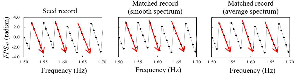
Figure 1. Fourier phase spectrum \([-\pi,\pi]\) of the seed and that of the matched records (component 2; smooth and average spectra). The dots indicate the fast Fourier transform (FFT) sampling points. The spectrum forms spiral patterns as shown by the red arrows. The patterns exist for frequencies up to 15 Hz for all three components and for all five records in Table 1. They were unaltered by the matching process (middle and right panels).
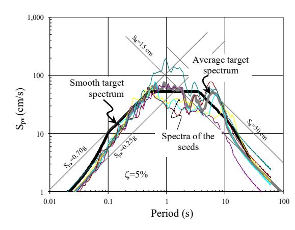
Figure 2. Smooth, five seed and average spectra (the average of the five seed spectra). Smooth spectrum was assumed, while the seed spectra were computed based on Eq. (2) for 5% damping.
PGAs were in the range of 0.19–0.33g. For each record, the displacement history was then computed using Eq. (2) for vector \(\mathbf{u}_{s}(t)\). The displacement spectrum was calculated as
\[S_{\mathbf{d}}(\omega,\zeta) = \max_{\mathbf{d}} \sqrt{u_{s1}^{2}(\omega,\zeta,t) + u_{s2}^{2}(\omega,\zeta,t) + u_{s3}^{2}(\omega,\zeta,t)}\] for \(\zeta = 5\%\). The pseudo-acceleration and pseudo-velocity spectra were computed as \(S_{p\mathbf{a}}(\omega) = \omega S_{p\mathbf{v}}(\omega) = \omega^2 S_{\mathbf{d}}(\omega)\), representing the three-component motions. All five spectra from the seeds were then averaged to form a second target, referred to as the average spectrum. Two spectral matchings were then performed against these two targets (smooth and average spectrum) which show different spectral ratio demand, and comparisons were made. The three-component seed records are listed in Table 1; their spectra are presented in Fig. 2. For the smooth spectrum, the target PGA and peak ground displacement (PGD) were 0.3g and 14.3 cm, respectively, while that of the average spectrum were 0.24g and 14.3 cm, respectively. A baseline correction was performed to all the acceleration data in Table 1 before spectral matching to ensure that the corresponding velocity and displacement time series were consistent and drift-free, with low-and-highfrequency distortions removed.
For illustration, the spectral matching of Chuetsu-oki (Japan, 2007, station Matsushiro Tokamachi, record ID 4843, the second row in Table 1) to the smooth and average spectra is now detailed. The accuracy of the matching procedure was measured based on the RMS error, expressed as (Suárez and Montejo, 2005, Hancock et al., 2006)
\[e = \sqrt{\frac{1}{n_e} \sum_{k=1}^{n_e} \left[ 1 - \frac{1}{P(k)} \right]^2}\] (19)
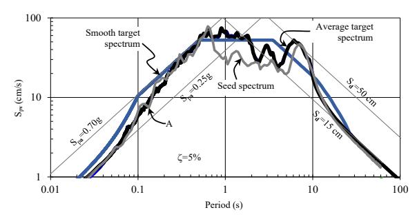
Figure 3. Smooth, seed, and average spectra. Notice the gaps between the smooth and average target spectra at low periods. At high periods the gaps are not that significant. Point A at periods 0.14 seconds (or frequency of approximately 7 Hz) produced the largest (smooth) spectral ratio.
where \(n_e\) is the number of data points within the frequency of interest (0.1–25 Hz).
The procedure involved the following steps: (1) The response spectral ratio of the target was computed with respect to the seed, P(T) = \[S_{pvt}(T)/S_{pvs}(T)\], where
\(S_{\rm pvt}(T)\) and \(S_{\rm pvs}(T)\) are the pseudo-velocity spectra of the target and seed records for 5% damping, respectively. (2) Refinement of P(T) was performed (see Shahbazian and Pezeshk (2010) for details). (3) Eq. (16)–(18) were used to obtain the modified ground accelerations with a specified \(\beta\). (4) A band-pass filter with a cut-off frequency of 0.1–25 Hz was applied to the modified record to remove noise (Press et. al., 2007). (5) The RMS error was calculated using Eq. (19), and the average of 1/P(T) over the frequency range of interest was computed. (6) The procedure was repeated when the error and the average value needed to be refined.
The response spectra of the targets (smooth and average) and of the seed record (Chuetsu-oki) are shown in Fig. 3. At high periods (low frequencies) the spectra are close one to the other, but the case is different at low periods (high frequencies). The seed and average spectra are close but not the seed and spectra. At frequencies higher than approximately 7 Hz, the spectral ratio is consistently higher for the smooth spectrum than for the average spectrum (see Fig. 8), consistent with the response spectrum shown in Fig. 3 for periods lower than 0.14 seconds (Point A). This resulted in higher spectral ratio demand for the smooth spectrum than those for the average spectrum. For the type of Chuetsu-oki earthquake record discussed herein, this produced less realistic vertical components compared to the seed. This could be fixed, however, when a scale factor is applied to the vertical component (see Eq. (18)).
The matching was performed for 6 and 9 iterations for the smooth and average target spectra, resulting in
<sup>3</sup>This spectrum is equivalent to the definition of RotD100, but for three-component records adopted herein (see for detail in Boore, 2010).
<sup>4</sup>The station was in the vicinity of the Kashiwazaki-Kariwa nuclear facilities.
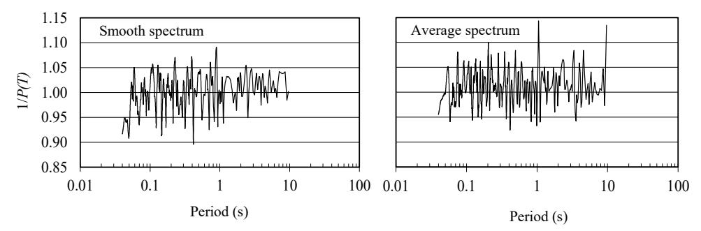
Figure 4. Reciprocal of the response spectral ratio of the matched record to that of the target, 1/P(T), mostly falling within the required range of 0.90–1.30 (ASCE/SEI, 2019). The average value was slightly above unity (1.005) for smooth target (left), and for average spectra (right).
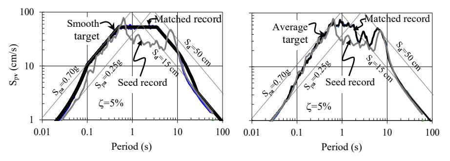
Figure 5. Target spectra for the spectral matching of Chuetsu-oki record. The pre- (grey line) and post-spectral (blue line) matching pseudo-velocity spectra are shown for 5% damping.
about 4% and 3% RMS error (computed by Eq. (19)), respectively. The reciprocal of the response spectral ratio (1/P(T)) is presented in Fig. 4, and most values fall in the specified range of 0.90-1.30 (ASCE/SEI, 2019), for the period range of 0.04-10 s. The average of 1/P(T) over the period of interest (0.04-10 s) was slightly above unity (1.005) for the smooth and average spectra, respectively, indicating a satisfactory matching process according to ASCE/SEI (2019). The response spectra before and after matching are shown in Fig. 5 for both targets. As expected, at low periods, the PGA converged to the spectral acceleration of around 0.27g and 0.22g; at high periods the PGD approached the spectral displacement of about 12.0 cm and 13.6 cm for the smooth and average spectra, respectively. Therefore, the matching produced a satisfactory convergence for periods 0.04–10 s, and the convergence for the smooth spectrum was fair at higher periods.
The accelerations, velocities, and displacements for the seed and matched records (both the smooth and average targets) are shown in Fig. 6. The scales among the components' accelerations look similar for the seed and matched time series (both for the smooth and average spectra). This was achieved by setting the scale factor for vertical component b=0.7 for the smooth and b=0.8 for the average spectra, respectively. The displacements look better for the smooth matched record than those for the average target. No drifts were observed in the velocity and displacement time series due to refinement process of P(T) in Step 2.
The amplitude of the frequency series direction cosines of the seed acceleration, \(|L_{aj}(f)|\) (j=1,2,3), as computed according to the equation that follows Eq. (18), are shown in Fig. 7 for three components. We observed that the direction cosine amplitudes of components -1 and -2 (horizontal) are dominant at frequencies lower than 7 Hz, while that of the vertical component is dominant at frequencies higher than approximately 18 Hz. Consequently, if a high spectral ratio demand is present at high frequencies, the vertical component will be driven more than the horizontal. This high spectral ratio demand at high frequencies was typical in the example considered herein and created too strong vertical components when they were not scaled down.
The Fourier amplitude spectral ratio between the modified and the seed records, as computed by Eq. (7), is shown in Fig. 8 for two target spectra (smooth and average). The ratio for the smooth spectrum was higher than that for the average target at frequencies higher than 7 Hz (or period 0.14 s or lower). This was due to a wider response spectral mismatch between the smooth target and the seed compared to that of the average spectra and the seed, at periods lower than about 0.14 s (observe Point A in Fig. 3); and this was typical for most of the seed records considered in the example (see Fig. 2). This higher spectral ratio demand for the smooth spectrum, together with the dominance of the vertical component direction cosines at high frequencies, drove the vertical component acceleration time series to unrealistic scales among the components;
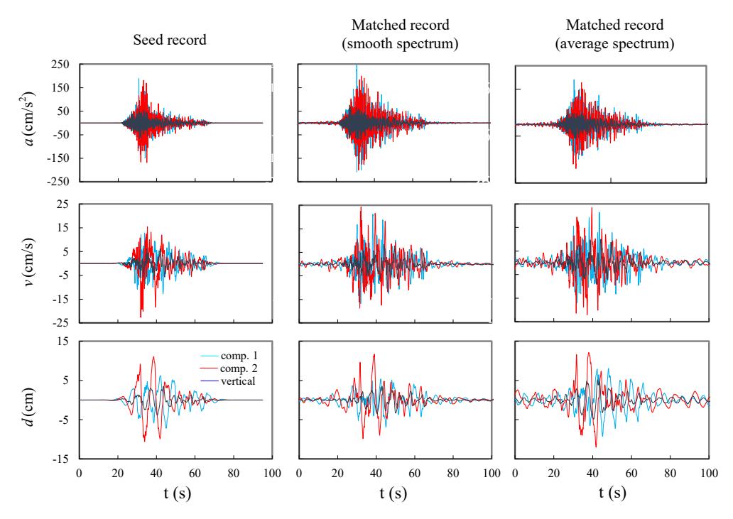
Figure 6. Accelerations, velocities, and displacements of the seed and matched records (both for the smooth and average spectra). Displacements (smooth target, mid panel) look better than that of the average spectrum. Vertical accelerations of the matched records look as realistic as the seed. Drifts were not observed in all records.
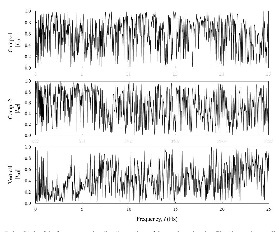
Figure 7. Amplitude of the frequency series direction cosines of the seed acceleration. Direction cosine amplitudes of the vertical component are relatively low at frequencies lower than 7 Hz and relatively high at frequencies higher than 18 Hz (bottom panel). This is different from those of the horizontal components which are Generally higher at lower frequencies (top and mid panels).
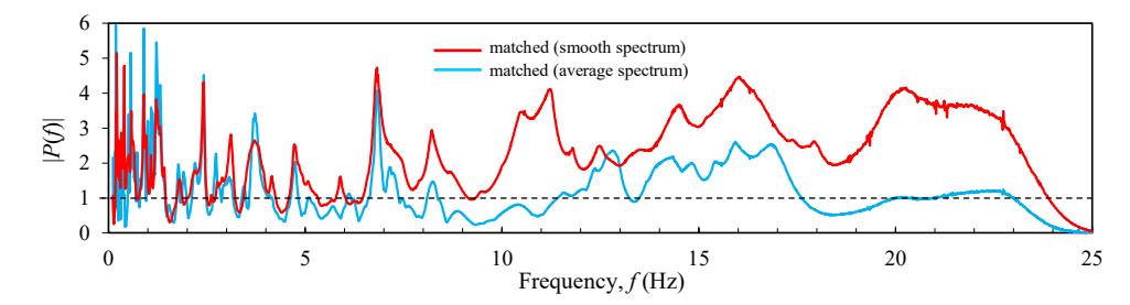
Figure 8. Fourier amplitude spectral ratio, |P(f)|, or the ratio of the FAS of the modified with respect to the seed records (see Eq. (7)). Notice the marked difference between them, especially at frequencies higher than 7 Hz.
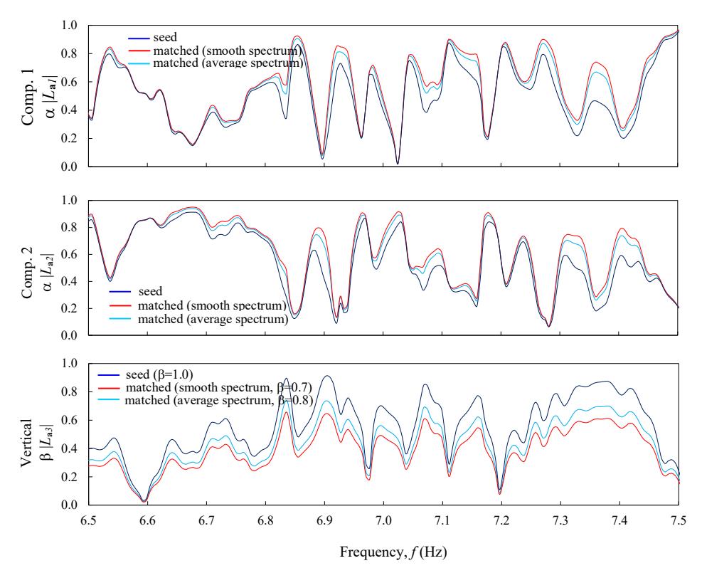
Figure 9. Amplitudes of frequency series direction cosines of three components after scaling; shown for frequencies 6.5–7.5 Hz. Vertical scale factor for the matched (smooth spectrum) was lower (\(\beta\)=0.7) than that of the average spectrum (\(\beta\)=0.8) because the spectral ratio demand of the former was higher than that of the latter (at high frequencies), where the direction cosines was dominated by the vertical component (see Fig. 7).
and this effect was resolvable by introducing a scale factor for the vertical component in Eq. (18). The effect of the scale factor on the direction cosines is presented in Fig. 9. The figure (bottom panel) shows that the matched vertical components (both smooth and average spectra) were scaled proportionally with respect to the seed's vertical component; however, the two horizontal components were scaled differently (see top and mid panels), consistent with Eq. (15). Moreover, the vertical component scale factor of the matched (smooth spectrum) was set lower than that for the average spectrum to produce realistic scales among the components because of the higher spectral ratio demand of the former (see bottom panel). The objective was to produce components scales of the modified records similar to that of the seed.
The Fourier amplitude spectra for the acceleration of the seed and matched records (FAS<sub>a</sub>) (for both the smooth and average spectra) are presented in Fig. 10. The comparisons as per components as well as the records show realistic scales among them. The matched (smooth target) record shows higher FAS values at higher frequencies is consistent with higher spectral ratio demands (shown in Fig. 8); as also consistent with the smooth spectral demand (see Fig. 3).
The resulting spectra for all five records are shown in Fig. 11 (left panel for smooth spectrum; right for average target). In general, the convergence was accurate up to periods of 10 s. This should be sufficient for most structural needs from stiff structures like nuclear confinements to the very flexible ones like long span bridges or tall building structures.
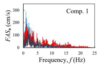
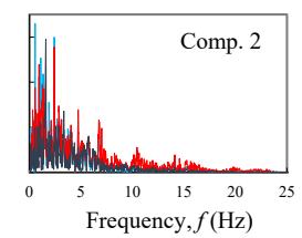
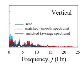
Figure 10. Fourier amplitude spectra of the acceleration of the seed and matched records (both smooth and average spectra). They look realistic (relative to the seed's) when comparing among the components and the records.
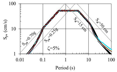
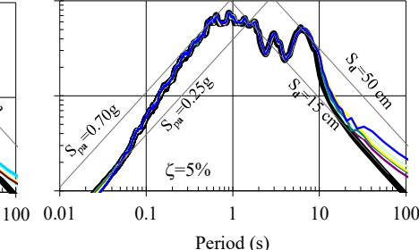
Figure 11 Pseudo-velocity spectra after spectral matching against the smooth (left panel) and average (right panel) spectra for all five seed records. All converge to the target up to periods of 10 s.
The modified time series were managed to have similar scales to those of the seeds by performing spectral scaling to the vertical components, as deemed appropriate. The need for vertical component spectral scaling varied depending on the nature of the seed and the spectral mismatch. In Table 1, Iwate seed (Semine Kurihara City station) did not require spectral scaling for its vertical component while Chi-Chi record (CHY034 station) required the lowest vertical component scale factor, \(\beta\)=0.6 and 0.7 for the smooth and average spectra, respectively. The former showed no dominance of the vertical component in the direction cosine amplitudes for the frequencies of interest, while the latter indicated the opposite situation. Other records employed vertical scale factors \(\beta\)=0.7 and 0.8 for the smooth and average spectra. In any case, using the vertical component scale factor produced three-component modified records with scales among their components similar to those of the seeds. Consequently, the directions cosines of three components were maintained.
4. Discussions
The three-component spectral matching outlined here avoided the complications that would have arisen otherwise. These include the correlation and synchronization issues among the components of the time series which might change the characteristics of the waveform entirely. As per ASCE/SEI (2019), for earthquake simulations, constructing three-component ground motions based on the individual components of seismic events require the three components to be statistically independent, indicated by the correlation coefficients being less than or equal to 0.16, for any pair. However, there are no regulations if the three-component motions are simultaneously generated based on a single event. As for the synchronizations, the issues should be thought of cautiously. Although the spectral matching procedure outlined above did not preserve the direction cosines of the seeds' time series, their interdependences were maintained. This is observed in Fig. 9 (or from Eqs. (16)-(18)), where the components' interrelations of the seed's frequency series are mathematically consistent. When the vertical component spectral scaling was not performed (\(\beta\)=1.0), the direction cosines of the frequency series were completely preserved (for the zero-phase filter, see Eq. (13)). Furthermore, if the spectral ratio filter function \(P(\omega)\), was constant then the time series direction cosines were conserved following the uniform spectral scaling for all components. Thus, components synchronizations are automatically taken care of by Eqs. (16)-(18).
5. Conclusions
The study can be summarized as follows:
1. A spectral matching of three-component seismic ground acceleration records was introduced. The procedure was applied in the framework of the Fourier transform and applicable to other eigenfunction expansion techniques. The three components were matched simultaneously so that the resulting spectrum agreed with a target; the target spectrum representing the three-component ground motion should be provided. The scales among the components of the modified records were maintained to be similar to those of the seeds to ensure that realistic three-component records could always be produced. This was achieved by performing spectral scaling to the vertical component simultaneously with the threecomponent spectral matching. The procedure
- prevented issues such as correlations and synchronizations among the components' time series.
- 2. The records modification was performed based on a filter function uniquely determined by the filter's amplitudes and phases. The amplitudes were computed based on the Fourier amplitude or the response spectra. When the former was utilized then the solution was straightforward, but if the latter was selected then an iteration scheme was necessary. The phases were arbitrary or could be set to specified values or zero. The former was used when a phase difference between the modified and seed was desired, while the latter was necessary when the spiral patterns of the records' phases needed to be maintained. The patterns were found in all five records considered in this paper for all three components for frequencies up to 15 Hz; it was also observed in other seismic events. The modified records with maintained phases were required in nonlinear response analyses of critical structures.
- 3. A refinement step was applied to the filter's amplitude to restore the accuracy of the acceleration records, thereby avoiding drifts in the velocity and displacement time series. Consequently, the convergence of the iteration and the accuracy of the resulting time series was enhanced.
- 4. The procedure resulted in drift-free time series and maintained components' scales as well as the phases. Such three-component time series with these properties is important in the nonlinear response analyses of critical structures, which are sensitive to three-component motions due to stiffness and/or mass irregularities. This cannot be achieved by the present procedures because they were mostly based onecomponent spectral matching processes.
Acknowledgement
The authors acknowledged the support of the Engineering Centre for Industry and the Centre for Infrastructures and Built Environment, both of Institute of Technology Bandung. The authors also gratefully acknowledged the constructive comments by the anonymous reviewer.
References
- Abrahamson, N.A. (1992) "Nonstationary spectral matching," Seismol. Res. Lett. 63(1), 30.
- Adekristi, A. and Eatherton, M.R. (2016) "Time-domain spectral matching of earthquake ground motions using Broyden updating," J. Earthq. Eng. 20(5), 679–698.
- Al Atik, L. and Abrahamson, N.A. (2010) "An improved method for nonstationary spectral matching," Earthq. Spectra 26(3), 601–617.
- ASCE/SEI (2019) "Seismic Design Criteria for Structures, Systems, and Components in Nuclear Facilities," ASCE/SEI Standard 43-19, American Society of Civil Engineers.
- Baker, J.W. and Lee, C. (2018) "An Improved Algorithm for Selecting Ground Motions to Match a Conditional Spectrum," J. Earthq. Eng. 22(4), 708-723.
- Bani-Hani, A.I. and Malkawi, K.A. (2017) "A multistep approach to generate response-spectrumcompatible artificial earthquake accelerograms," Soil Dynam. Earthq. Eng. 97, 117-132.
- Boore, D.M. (2010) "Orientation-independent, nongeometric - mean measures of seismic intensity from two horizontal components of motion," Bull. Seismol. Soc. Am. 100(4), 1830–1835.
- Carlson, C., Zekkos, D. and Athanasopoulos-Zekkos, A. (2016) "Predictive equations to quantify the impact of spectral matching on ground motion characteristics," Earthq. Spectra 32(1), 125–142.
- Chopra, A.K. (2020) "Dynamics of Structures: Theory and Applications to Earthquake Engineering," 5th ed. in SI Units, Pearson (USA), pp. 331-377.
- Clough, R.W. and Penzien, J. (2003) "Dynamics of Structures," 3rd ed., Computers & Structures, Inc., USA.
- Gao, Y., Wu, Y., Li, D., Zhang, N. and Zhang, F. (2014) "An Improved Method for the generating of Spectrum-Compatible Time Series Using Wavelets," Earthq. Spectra 30(4), 1467–1485.
- Gasparini, D.A. and Vanmarcke, E.H. (1976) "SIMQKE: Simulated Earthquake Motions Compatible with Prescribed Response Spectra," Department of Civil Engineering, Res. Rep., Massachusetts Institute of Technology (Cambridge, Massachusetts) 65 pp. R76–4.
- Hancock, J., Watson-Lamprey, J., Abrahamson, N.A., Bommer, J.J., Markatis, A., McCoy, E. and Mendis, R. (2006) "An improved method of matching response spectra of recorded earthquake ground motion using wavelets," J. Earthq. Eng. 10(sup001), 67–89.
- Hudson, D.E. (1962) "Some problems in the application of spectrum techniques to strong motionearthquake analysis," Bull. Seismol. Soc. Am. 52(2), 417–430.
- Kaul, M. K. (1978) "Spectrum-consistent Time-History generation," J. Eng. Mech. Div. (ASCE) 104(4), 781–788.
- Kohrangi, M., Bazzurro, P., Vamvatsikos, D. and Spillatura, A. (2017) "Conditional spectrumbased ground motion record selection using average spectral acceleration," Earthquake Eng. Struct. Dyn. 46(10), 1667–1685.
- Kost, G., Tellkamp, T., Kamil, H., Gantayat, A. and Weber, F. (1978) "Automated generation of
- spectrum-compatible artificial time histories," Nucl. Eng. Des. 45(1), 243–249.
- Li, B., Ly, B.L., Xie, W.C. and Pandey, M.D. (2017) "Generating spectrum-compatible time histories using eigenfunctions," Bull. Seismol. Soc. Am. 107(3), 1512-152.
- Li, B., Xie, W.C. and Pandey, M.D. (2016) "Generate tri-directional spectra-compatible time histories using HHT method," Nucl. Eng. Des. 308, 73–85.
- Lilhanand, K. and Tseng, W.S. (1988) "Development and application of realistic earthquake time histories compatible with multiple damping response spectra," Proc. of the Ninth World Conference on Earthquake Engineering, Tokyo, Japan, Vol. 2, pp. 819–824.
- Mukherjee, S. and Gupta, V. K. (2002) "Waveletbased characterization of design ground motions," Earthquake Eng. Struct. Dyn. 31(5), 1173–1190.
- Ni, S.H., Xie, W.C. and Pandey, M.D. (2011) "Tridirectional spectrum-compatible earthquake time-histories for nuclear energy facilities," Nucl. Eng. Des. 241(8), 2732–2743.
- Ohsaki, Y. (1979) "On the significance of phase content in earthquake ground motions," Earthquake Eng. Struct. Dyn. 7(5), 427–439.
- PEER (2022) "Ground Motion Database," Pacific Earthquake Engineering Research Center https://ngawest2.berkeley.edu/spectras/new? sourceDb_flag=1 (last accessed August).
- Press, W.H., Teukolsky, S.A., Vetterling, W.T. and Flannery, B.P. (2007) "Numerical Recipes: The Art of Scientific Computing," 3rd ed., Cambridge University Press (New York, USA), pp. 600- 602.
- Preumont, A. (1984) "The generation of spectrum compatible accelerograms for the design of nuclear power plants," Earthquake Eng. Struct. Dyn. 12(4), 481–497.
- Rizzo, P.C., Shaw, D.E. and Jarecki, S.J. (1975) "Development of real/synthetic time histories to match smooth design spectra," Nucl. Eng. Des. 32(1), 148–155.
- Shahbazian, A. and Pezeshk, S. (2010) "Improved velocity and displacement time histories in frequency domain spectral-matching procedures," Bull. Seismol. Soc. Am. 100(6), 3213-3223.
- Silva, W. J. and Lee, K. (1987) "WES RASCAL code for synthesizing earthquake ground motions," Report 24. Misc. Paper S-73-1, Department of the Army (US Army Corps of Engineers) pp. S-73–71.
- Suárez, L.E. and Montejo, L.A. (2005) "Generation of artificial earthquakes via the wavelet transform," Int. J. Solids Struct. 42(21-22), 5905–5919.
- Tao, D., Lin, J. and Lu, Z. (2019) "Time-frequency frequency energy distribution of ground motion and its effect on the dynamic response of nonlinear structures," Sustainability 11(3), 702.
- Thrainsson, H., Kiremidjian, A.S. and Winterstein, S.R. (2000) "Modeling of earthquake ground motion in the frequency domain," Report No. 134, The John A. Blume Earthquake Engineering Centre, Department Civil and Environmental Enginering (Stanford University, Stanford, California).
- Tiliouine, B., Hammoutene, M. and Bard, P.Y. (2000) "Phase angle properties of earthquake strong motions: A critical look," Proc. of the Twelfth World Conference on Earthquake Engineering, Auckland, New Zealand.
- Wang, G., Youngs, R., Power, M. and Li, Z. (2014) "Design ground motion library (DGML): An interactive tool for selecting earthquake ground motions," Earthq. Spectra 31, 617–635.
- Yang, L., Xie, W.C., Xu, W., Ly, B.L., Liu, W. and Li, W. (2021) "Generation of Tri-Directional Spectra-Compatible Time Histories Coupling the Influence Matrix Method and Gram– Schmidt Orthogonalization," Int. J. Struct. Stab. Dyn. 21(13), 2150186 1-27.