
1. Introduction
A river is a natural or artificial water channel container which is in the form of a water drainage network from the upstream to the estuary, has right and left boundaries by borderlines (Permen PUPR, 2015 No. 28/PRT/M/2015). Bangga River is a river in Palu City that located in mountainous area. On February 29 and April 21, 2019, the flood in this river flowed through Bangga Villages, Sigi Regency, Palu City, Central Sulawesi Province. It can be shown in Figure 1. The flood carried sediment material, such as sand, rocks, and woods. On September 28, 2018, Palu Earthquake caused tremendous damage to the coastal area of Palu, Central Sulawesi, Indonesia (Sihombing, at, al., 2020). The flood and earthquake cause sediment buildup in Bangga River. The potential of sediment is about 13,350,000 m3 . Based on the condition, the Ministry of Public Works and Housing through BWS Sulawesi III do the river improvement and sediment control to reduce the risk of flooding caused by sediment, increase river capacity, strengthen riverbanks and
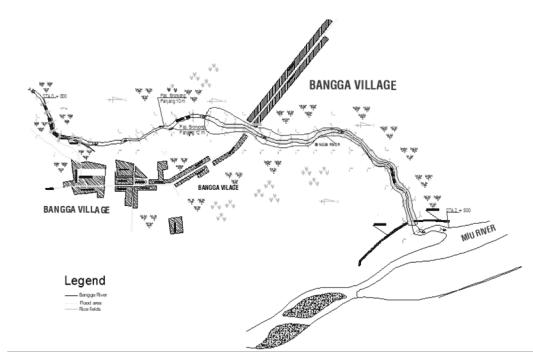
Figure 1. Flood area in Bangga watershed
reduce the amount of sediment in the Bangga River. Hence, the limitation of this study aims to analyze the performance of sediment control in reducing the flood and sediment total only in Bangga Watershed.
2. Study Area
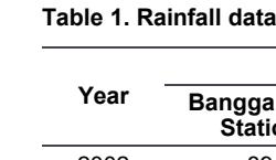
This study was carried out in Bangga River, located on theWest of the Palu River. The lower of Bangga River form an alluvial fan area around the Palu River which is used as residential areas and rice fields (Fauzan, at, al., 2021). The length of Bangga River is 17.33 km and 74.92 km2 of area. The upstream slope is +0.05 and the downstream slope is +0.01. The river width is 9.29 m in upstream, 47.6 m in the middle stream, and 29.25 m in the downstream. Bangga Watershed contains two sub-watersheds. The study area can be seen in Figure 2.
| HHMT | |||
|---|---|---|---|
| Year | Bangga Atas Station | Bangga Bawah Station | Tuva Station |
| 2002 | 89 | 95 | 98 |
| 2003 | 49 | 46 | 80 |
| 2004 | 70 | 65 | 78 |
| 2005 | 52 | 33 | 88 |
| 2006 | 67 | 72 | 91 |
| 2007 | 79 | 87 | 100 |
| 2008 | 72 | 58 | 91 |
| 2009 | 98 | 50 | 93 |
| 2010 | 111 | 77 | 97 |
| 2011 | 96 | 80 | 65 |
| 2012 | 61 | 40 | 87 |
| 2013 | 63 | 61 | 109 |
| 2014 | 103 | 40 | 77 |
3. Materials and Methods
Primary and secondary data collection was carried out to analyze supporting data. The primary data collected includes: grain size, unit weight, and sediment concentration in five samples taken from Bangga River. Secondary data were obtained from previous studies and related Institutions. Hydrology analysis using rainfall data from three rainfall station (Bangga
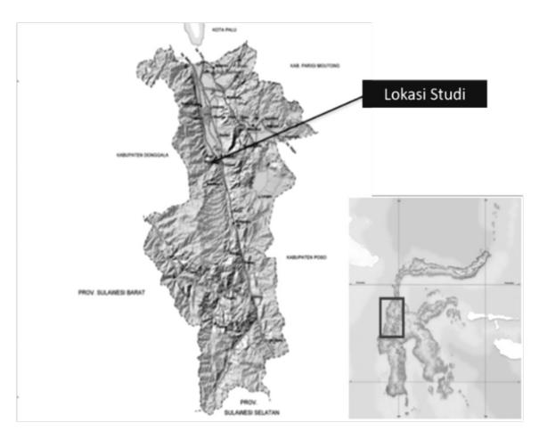
Figure 2. The study area of this research
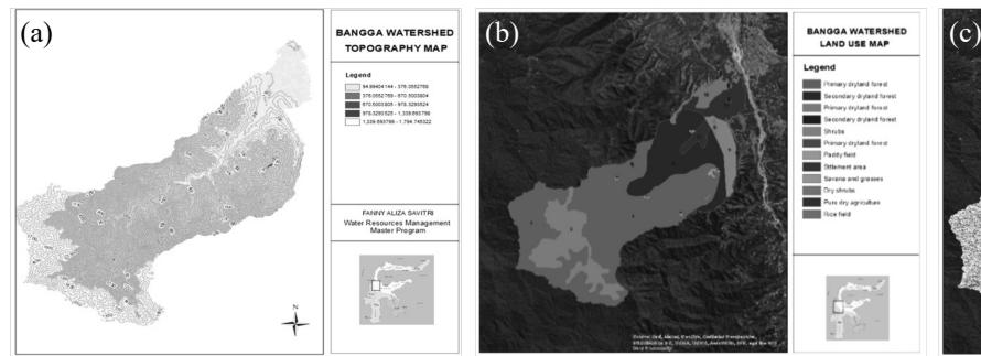
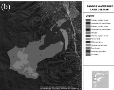
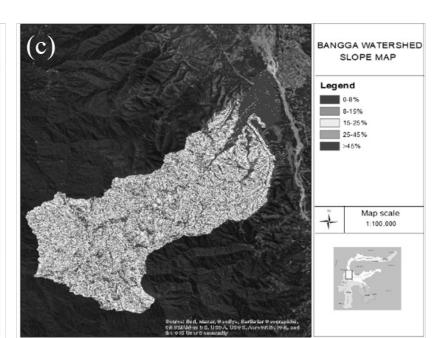
Figure 3. Topography (a) (b) Land use (c) Slope
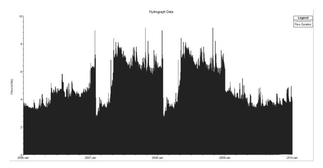
Figure 4. Daily discharge
Atas, Bangga Bawah, and Tuva) on 14 years from 2002 to 2014, daily discharge on 4 years on 2006 to 2009, topography data from Digital Elevation Model (DEM), land use map from Ministry of Environment and Forestry, and also soil data from Harmonized World Soil Database (HWSD). The land map will analyze to obtain the runoff coefficient and Manning's n value for the inflow discharge hydrograph (Yakti, at, al., 2018). Figure 3 shows the topography map, land use map and slope map from Bangga Watershed. The average slope map provides information on slope distribution over the entire basin and slope maps play a crucial role in addition to flow direction and flow accumulation in hydrological modeling (Eadara, Karanam, 2013). The majority of the slope on this watershed is 15-25% and has an area 22.41 km<sup>2</sup>. The rainfall data are shown in Table 1, and daily discharge data are shown in Figure 4.
The rainfall data is used for flood discharge design. Daily discharge data is for sediment transport simulation using Engelund-Hansen, Meyer Peter Muller (MPM), and Yang's formula. The hydrological analysis consists of watershed delineation from topographic conditions and rainfall area analysis using Thiessen Method.
Thiessen is a simple and straight forward method, each interpolated location is given the value of closest measurement point and resulting in a typical polygonal pattern (Buytaert, at al., 2006) Hence, the flood frequency analysis was carried out using 3 statistical methods using historical rainfall data which are Normal, Gumbel, Log Normal and Log Pearson III (Jaya, at al.), and HEC-RAS used analysis flood discharge. HEC model is designed to simulate the surface runoff response of a catchment to precipitation by representing the catchment with interconnected hydrologic (Bronswijk, at, al., 1995), and design flood with Synthetic Unit Hydrograph (SUH) namely Soil Conservation Service and Snyder (BSN, 2016). Analysis of flow pattern and sediment transport with HER-RAS 1D Software with unsteady flow condition. The boundary upstream is a 100-years return period of flood discharge design and daily discharge on 4 years. The sediment modeling on upstream using rating curve of sediment concentration and the downstream boundary is normal depth. Modeling is carried out under two conditions, existing conditions and conditions after sediment controllers building. The analysis is to determine the rate of the infrastructure to control the sediment transport. Several types of controller infrastructure are sabo dams, check dams and groundsill. The former is generally a wall-type structure. It is designed to elevate the torrent bed to fix and stabilize the bottom profile (Chanson, 2004).
Table 2. Thiessen area for Bangga watershed
| Sub watershed | |||||
|---|---|---|---|---|---|
| No | Bangga Atas | Bangga Bawah | Tuva | Total | |
| 1 | AWLR | 58.31 | 1.86 | 4.58 | 60.2 |
| 2 | Hilir | 5.35 | 9.22 | 0.09 | 14.66 |
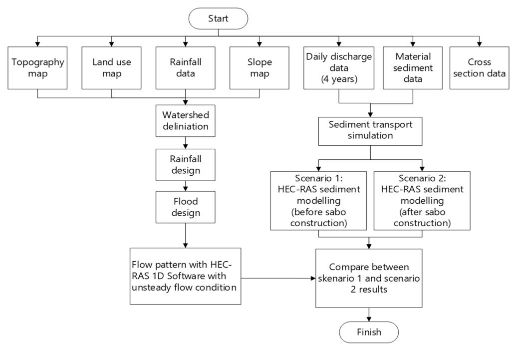
Figure 5. Research flowchart
Table 3. Design rainfall in AWLR sub watershed
| N. | Detum Devied (T) | Design Rainfall (mm) | |||||
|---|---|---|---|---|---|---|---|
| No | Return Period (T) — | Normal | Gumbel | Log Normal | Log Pearson III | ||
| 1 | 2 75.56 72.44 | 73.30 | 74.12 | ||||
| 2 | 5 | 91.55 | 89.24 | 91.20 | 91.43 | ||
| 3 | 10 | 99.92 | 100.36 | 102.24 | 101.42 | ||
| 4 | 25 | 108.84 | 114.41 | 115.49 | 112.77 | ||
| 5 | 50 | 114.60 | 124.83 | 124.95 | 120.47 | ||
| 6 | 100 | 119.79 135.18 | 134.11 | 127.64 | |||
| 7 | 200 | 124.53 | 145.49 | 143.08 | 134.40 | ||
| 8 1000 | 134.30 | 169.37 | 163.52 | 148.90 | |||
| 0.092 | 0.058 | 0.094 | 0.076 | ||||
| Smirno | ov Kolmogorov Test | 0.368 | 0.368 | 0.368 | 0.368 | ||
| - | accepted acce | accepted | accepted | ||||
| Chi-Square Test | 1.231 | 1.231 | 2.000 | 1.231 | |||
| Chi-Square Test 5.991 | 5.991 5.991 | ||||||
| accepted | accepted | accepted | accepted | ||||
Table 4. Design rainfall in downstream sub watershed
| No | Deturn Deried (T) | Design R | ainfall (mm) | |||
|---|---|---|---|---|---|---|
| NO | Return Period (T) - | Normal | Gumbel | Log Normal | Log Pearson III | |
| 1 | 2 91.00 85.77 | 86.21 | 85.11 | |||
| 2 | 5 | 117.80 | 113.92 | 114.79 | 114.27 | |
| 3 | 10 | 131.83 | 132.56 | 133.34 | 134.32 | |
| 4 | 25 | 146.78 | 156.10 | 156.43 | 160.50 | |
| 5 | 50 | 156.43 | 173.57 | 173.42 | 180.64 | |
| 6 | 100 | 165.12 | 190.92 | 190.28 | 201.33 | |
| 7 | 200 | 173.06 208.19 207. | 207.14 | 222.74 | ||
| 8 | 1000 | 189.44 | 248.22 | 246.75 | 275.88 | |
| , | 0.116 | 0.083 | 0.104 | 0.107 | ||
| Uji Smii | mirnov-Kolmogorov Test 0.3680 | 0.3680 | 0.3680 | 0.3680 | ||
| accepted | accepted | accepted | accepted | |||
| , | 3.615 | 2.000 | 2.000 | 2.000 | ||
| Uji | Chi-Square Test | 5.9910 | 5.9910 5.9910 | 5.9910 | ||
| accepted | accepted | accepted | accepted | |||
4. Results and Discussions
4.1 Rainfall analysis
Watershed area from Geographic Information System (GIS) Software is used for rainfall area analysis. After that, the rainfall area and the abstraction of rainfall can be obtained. The Automatic Water Level Recorder (AWLR) sub watershed area is 60.2 km² and 14.66 km² of downstream sub-watershed. The result of sub-watershed area analysis can be seen in Table 2. Meanwhile, the design rainfall distribution analysis using Gumbel and Log Pearson III methods have the best results, and the normality tests are Chi-Square and Smirnov Kolmogorov (Yazici, Yolacan,2007). The results of the design rainfall analysis described in Table 3 and Table 4.
4.2 Design discharge
The hydrological analysis is divided into two subwatersheds are the downstream and AWLR. Maximum
rainfall design data was obtained from 3 rainfall stations for 14 years of data (2002-2014). The analysis uses SCS and Snyder with the hydraulic input data is 100-year return period. The analysis result shows that the flood discharge design of the 100-year return period from the SCS method in the AWLR subwatershed is 124.6 m³/s and 107 m³/s from Snyder. Meanwhile, in downstream sub-watershed from the SCS method is 44.2 m³/s and 86.9 m³/s from Snyder. The diagram shows in Figure 5.
4.3 Hydrology data calibration
The calibration of return period flood discharge using bankfull capacity discharge. The bankfull discharge was defined as the discharge which filled the channel to the level of the floodplain (Andrews, 1980). The cross section used for calibration is Sta 194 in AWLR location with the natural channel condition. Manning's formula is widely used in hydrology, hydraulics, irrigation etc (Bonetti, 2017). The Manning value is 160 Jurnal Teknik Sipil
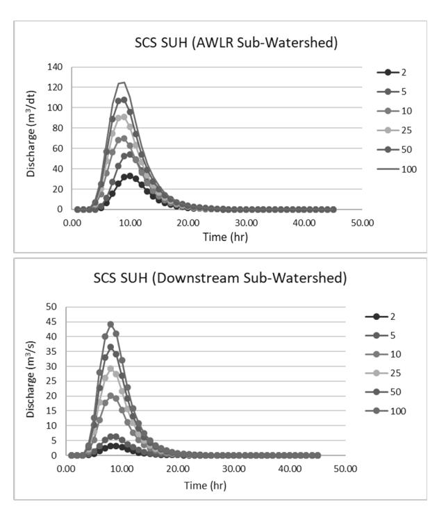
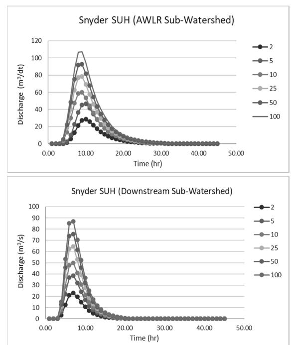
Figure 6. (a) SCS-SUH AWLR sub watershed (b) snyder SUH AWLR sub watershed (c) SCS-SUH downstream sub watershed (d) snyder SUH downstream sub watershed
0.07, which means the channel's type is mountainous river that consist of grave and big rocks (Nasional, at al., 2008) The condition is same with the existing condition. The equation to analyze the bankfull discharge formula be seen in the equation below:
\[Q = \frac{1}{n} R^{\frac{2}{3}} S^{\frac{1}{2}} A = \frac{1}{0.07} \left( \frac{13.315}{11.257} \right)^{\frac{2}{3}} (0.024)^{\frac{1}{2}} = 32.958 \text{ m}^3/\text{s}\] (1)
In this equation, Q is bankfull discharge (m3 /s), n is Manning's roughness parameter. R is hydraulic radius (m), S is bed slope and A is channel cross sectional area (m).
Based on the calculations with SCS and Snyder, it was found that the value close to the bankfull discharge is from the SCS method, which 33.1 m3 /s (2-year return period). So that the method to analyze and for input data of flood discharge design is using SCS method with the time lag is 260 minutes (4.33 hours).
4.4 Hydraulic model analysis
The hydraulic analysis is carried out for runoff modeling in Bangga River in existing and sabo dam condition. The modeling is used HEC-RAS, which was made by the Hydrologic Engineering Center (HEC) from the US Army Corps of Engineers (USACE). Hydraulic models in HEC-RAS are typically calibrated against Manning's roughness (Environmental, 2016). The research uses is unsteady 1D with the cross-section data is from 2019th , containing of Sta 0 to Sta 194. The first modeling is existing condition was carried out on the main river, which downstream sub-watershed as the boundary of lateral inflow hydrograph. The normal depth is 0.0158. The second model is to add 3 sabo dams. The first type of sabo dam is a slit that take place on Sta 152.5. Second sabo is open type in Sta 118.25 and the third sabo is also
Table 5. Recapitulation of peak discharge
| Return Period | Peak Disharge (m3 /s) | ||||
|---|---|---|---|---|---|
| No | (th) | SCS | Snyder | ||
| 1 | 2 | 33,1 | 29 | ||
| 2 | 5 | 54,1 | 47 | ||
| 3 | 10 | 69,7 | 59 | ||
| 4 | 25 | 90,8 | 78 | ||
| 5 | 50 | 107,5 | 93 | ||
| 6 | 100 | 124,6 | 107 | ||
Figure 7. Long section in existing condition
open type on Sta 72.5 with 11 m height and 14.3 m width and there are 4 slits on 2 m of height. The top elevation of sabo is +161 m, and the open channel is on +150 m. The other sub dams is on +146.4 m. Sabo 2 is a conduit type sabo with a width of + 45.17 m and a height of + 11 m and has 5 holes in the body of the sabo with each diameter of 1 m. Likewise, sabo 3 has a height ranging from + 13.5 to 14.5 m with a total of 5 holes with a diameter of 1 m.
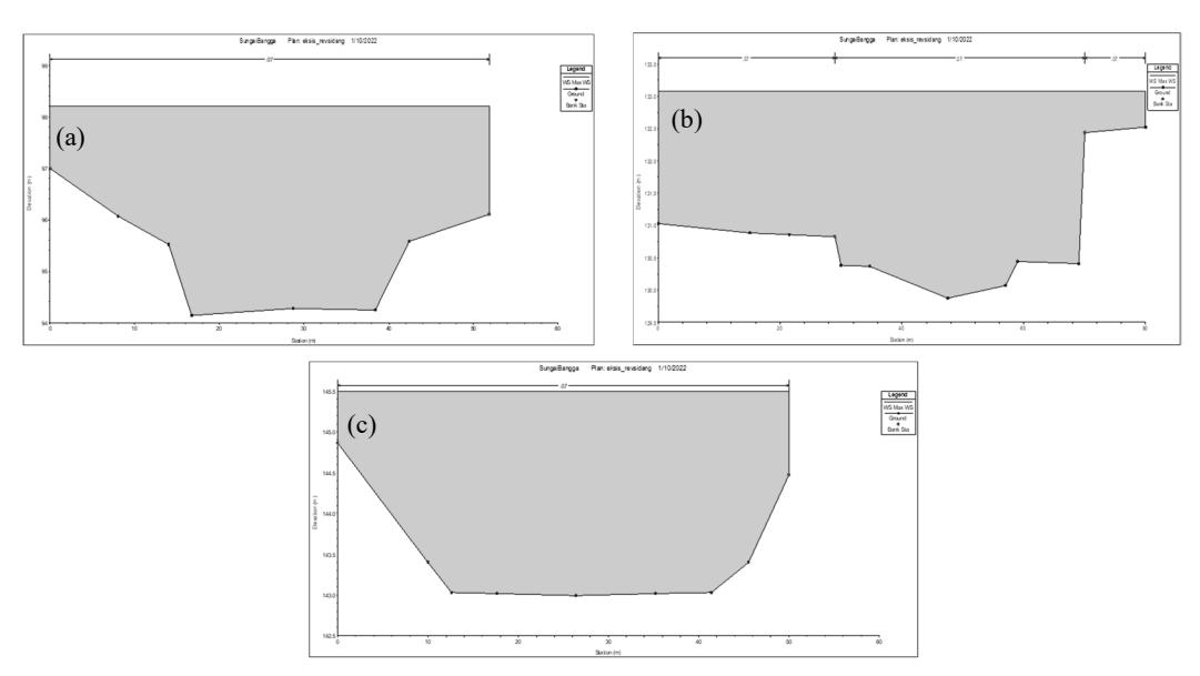
Figure 8. Cross section of existing (a) downstream (b) middle stream (c) upstream
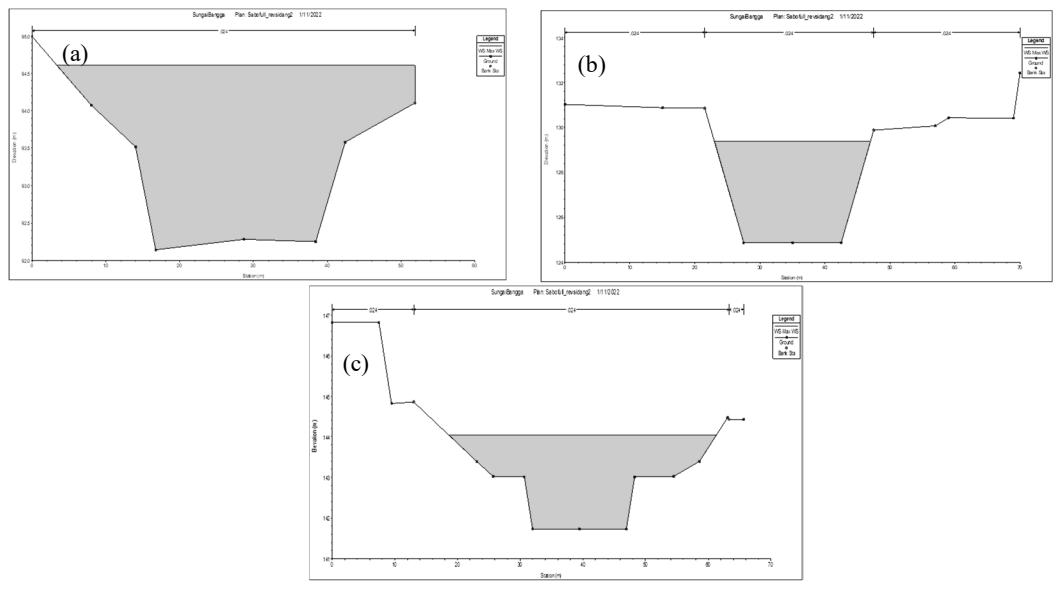
Figure 10. Cross section of after sabo (a) downstream (b) middle stream (c) upstream
The 100-year return period of modeling result shows that on existing condition, on Sta 2 (downstream) the runoff is 2.12 m. On the middle stream (Sta 113), the runoff is 2.25 m, and on the upstream is 0.62 m.
The runoff on Sta 2 is calibrated with historical data, which the flood of Bangga River was 2 to 3 m of height (Bonetti, at al., 2017). Meanwhile, the result of modeling by adding sabo dams shows that there is no runoff on Sta 2, Sta 113, and Sta 148. It means that the sabo dams can reduce the runoff in Bangga River by 100%.
4.5 Comparison of existing hydrograph and after sabo
According to the HEC-HMS simulation, it was found that the difference in peak discharge from the existing condition and after three sabo's bulding at 100 years return period. The peak discharge of the existing HSS
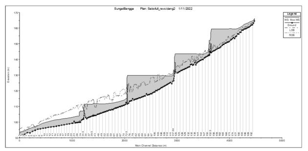
Figure 9. Long section in sabo condition
was 124.6 m³/s with a peak time (Tp) at 8 hours and HSS Sabo had a peak discharge of 93.8 m³/s with peak time at 12 hours. Figure 9 it shown that the time lag is a four hours slowdown due to the sabo blocking the flow of flood discharge going downstream.
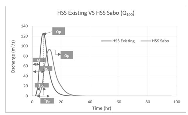
Figure 11. Graph of comparison of existing hydrograph and after Sabo
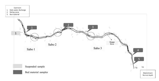
Figure 12. Sediment transport analysis modelling scheme
4.6 Sediment transport analysis
The concept of sediment transport capacity is commonly used in modelling sediment movement via overland flow and in channel transport models (Merritt, at al., 2003). This research employed the quasi unsteady sediment transport analysis module for sediment transport simulation (Environmental, 2016). Different processes of sediment transport can affect a single stream, depending on changes in sediment availability (i.e., sediment sources and their connectivity) and water runoff induced by a specific hydrological event (Brenna, at al., 2020). The sediment transport analysis is similar with the hydraulic analysis, but the input data is using daily discharge of 2006-2009.
The sediment data is the field data from 5 sampling points. Based on Laboratory analysis, the result of material are sand and silt. Sand or silt flows involving significant pore-pressures tend to occur in certain welldefined. These include submerged deposits of loose deltaic sand (Hungr, at al., 2001). The other boundary condition is using floating sediment rating curve. Sediment rating curves should be develop on seasonal basis to evaluate impacts of seasonal differences in sediment source pathway dynamics (Pickering, Ford, 2021).
4.6.1 Existing condition analysis
The sediment transport modeling uses Engelund Hansen, MPM and Yang due to the existing granular material from Laboratory test results > 15 mm for d50. The results of sediment transport modeling using Engelund Hansen formula show that the average degradation in the middle at Sta 76 is as high as 3.8 m due to the steep slope of the
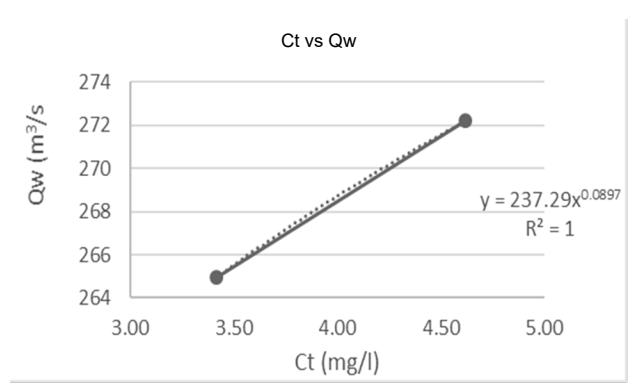
Figure 13. Graph of relationship between discharge and concentration in Bangga river
channel and the flow velocity that occurs in the middle of the river. The point increases, which results in scouring at the bottom of the channel. Meanwhile towards the downstream direction, there is an aggradation of 4.19 m at Sta 66. Aggradation occurs at a point where the slope is flatter than upstream so that the flow velocity is low and results in the deposition of particles carried from the upstream to Sta 66. Sedimentary deposits result from a long and complex history of aggradation and degradation cycles related to the changing nature of environmental controls affecting the sediment and water regimes of the catchment (Bertrand, at al., 2013).
According to Table 6, the amount of sediment from Sta 4 (downstream) is 409,709 ton/ 4years and from Sta 114 (middle stream, after sabo 1 and sabo 2) is 265,658 ton/ 4years. While on the upstream (Sta 185) is 27062 ton/ 4years
Table 6. Sediment total in existing condition
| No | River Sta | Sediment Total (ton/ 4 years) |
|---|---|---|
| 1 | 4 | 409,709 |
| 2 | 71 | 308,618 |
| 3 | 114 | 26,565 |
| 4 | 148 | 111,751 |
| 5 | 185 | 27,062 |
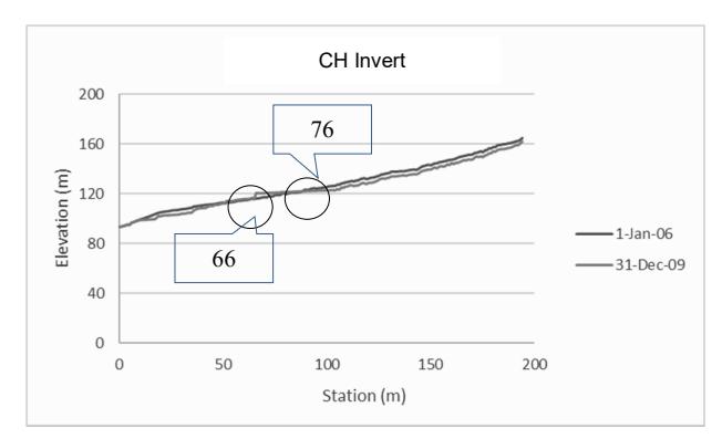
Figure 14. Invert elevation in existing condition
4.6.2 After sabo dams condition analysis
Based on the results of modeling using 3 (three) sabos using the Engelund-Hansen formula, it was found that the significant degradation occurred in the upstream part of the sabo as high as 3.8 m, namely at Sta 178. While the aggradation occurred before sabo 1 was 2.8 m high, sabo 2 was 1.39 m high and sabo 3 was as high as 0.084 m and the maximum aggradation is at Sta 80 which is 5 m high. In this zone, sediment originating from upstream in the presence of a structure across the river causes deposit to be retained and captured by the building and distributed downstream into scouring until it reaches a stable condition.
a. Engelund and Hansen
Engelund and Hansen formula selected for comparison developed based on flume data, using sediment size of bed material as input (WU, at al., 2008).
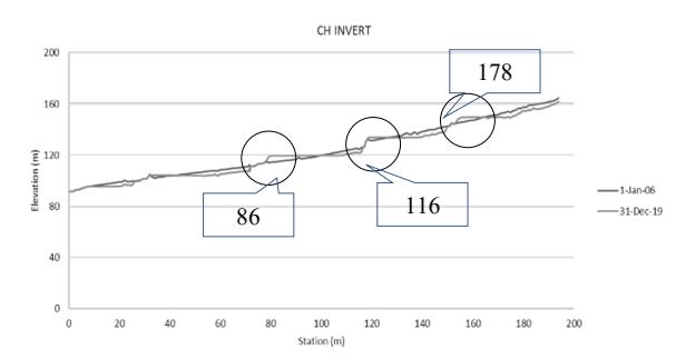
Figure 15. Invert elevation in Engelund-Hansen formula
Table 7. Sediment total in Engelund-Hansen
| No | River Sta | Sediment Total (ton/ 4 years) |
|---|---|---|
| 1 | 4 | 76,383 |
| 2 | 71 | 3,471 |
| 3 | 114 | 29,068 |
| 4 | 148 | 3,688 |
| 5 | 185 | 26,298 |
According to Table 7, the sediment from Sta 4 is 76,383 ton/ 4 years (409,709 ton/ 4years before). So the sabo dam can reduce the sediment transport is 81%. Meanwhile, on Sta 114 the sediment reduced by 89%, and on Sta 185 is 3%.
b. Meyer Peter Muller (MPM)
MPM was found to perform reasonably well by Gomez and Church [22]. A total sediment transport curve was constructed for each gaging station by adding measured instantaneous suspended sediment discharge to bedload sediment discharge computed by MPM [12]. The formula analysis shows that the maximum degradation is at Sta 178 as high as 3.99 m. Meanwhile, the largest aggradation is at Sta 86 is 3.85 m.
Based on Table 8, the results of total sediment at Sta 4 downstream was 31,816 tons / 4 years, in sta 114 (middle stream) is 8,465 tons/4 years, and in Sta 185
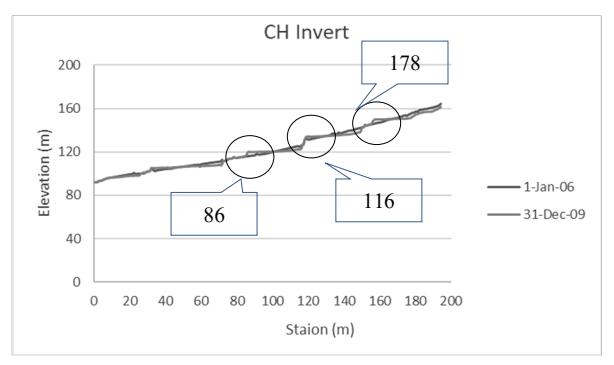
Figure 16. Invert elevation in Meyer Peter Muller formula
Table 8. Sediment total in Meyer-Peter Muller
| No | River Sta | Sediment Total (ton/ 4 years) |
|---|---|---|
| 1 | 4 | 31,816 |
| 2 | 71 | 1,620 |
| 3 | 114 | 8,465 |
| 4 | 148 | 3,661 |
| 5 | 185 | 27,668 |
(upstream) is 27,688 tons/4 years. While in MPM simulation, the reduction of the total sediment at Sta 4 by 92%, Sta 114 by 98%, and Sta 185 by 3%.
c. Yang
Yang's formula were selected for comparison using sediment size and suspended load as input [21]. Based on the analysis results, the formula shows the maximum degradation is at Sta 178 as high as 3.99 m. Meanwhile, the largest aggradation is at Sta 86, which is 3.85 m.
According to Table 9, the results of total sediment at Sta 4 (downstream) was 33,461 tons / 4 years and 114 (middle stream and coincided with the location of the
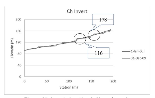
Figure 17. Invert elevation in Yang formula
Table 9. Sediment total in Yang
| No | River Sta Sediment Total (ton/ 4 years) | ||||
|---|---|---|---|---|---|
| 1 | 4 | 31,816 | |||
| 2 | 71 | 1,620 | |||
| 3 | 114 | 8,465 | |||
| 4 | 148 | 3,661 | |||
| 5 | 185 | 27,668 | |||
Table 10. Sediment transport simulation
| Engelund Hansen | Meyer Peter Muller | Yang | |||||||
|---|---|---|---|---|---|---|---|---|---|
| Average Region | Max Degradation | Max Agradation | Total Sediment | Max Degradation | Max Agradation | Total Sediment | Max Degradation | Max Agradation | Total Sediment |
| (m) | (m) | (ton/ 4 years) | (m) | (m) | (ton/ 4 years) | (m) | (m) | (ton/ 4 years) | |
| Upstream | -3.99 | 3.89 | 26298 | -4.00 | 3.66 | 27669 | -4.00 | 3.54 | 23339 |
| Middle Stream | -3.79 | 5.25 | 29069 | -4.00 | 3.85 | 8465 | -3.99 | 4.02 | 10483 |
| Down Stream | -3.58 | 2.25 | 76383 | 2.75 | -2.63 | 31816 | -2.73 | 2.75 | 33461 |
point after the placement of sabo one and sabo 2). is 10,483 tons/4 years, and 185 (upstream) is 23,339 tons/4 years. So, this formula can reduce sediment total at Sta 4 by 91.8%, Sta 96.1%, and at Sta 185 by 13.8%. This simulation was carried out using the same river geometry as hydraulic analysis and using 3 (three) transport functions, namely Engelund Hansen, Meyer Peter Muller, and Yang formulas. The summary of the analysis will present in the following table:
The table shows the river's degradation and aggradation in river morphology using the Yang and MPM equations has relatively the same results for all parts of the river. Yang's formula is more signifficant to reduce sediment total, in the upstream are able to reduce total sediment by upstream 13%, middle stream 96.1% and downstream 91.8%.
5. Conclusion
The conclusions of this research are:
- 1. Bankfull discharge of the Bangga River is 32.95 m3 /s and equivalent to a 2-year return discharge using the HSS SCS method, which is 33.1 m3 /s.
- 2. The results of the HEC-RAS 1D simulation, which uses two conditions existing and after the sabo dam's was built, show that the water surface is stood at 2.1 m depth before the constructed sabo dam. However, the simulation indicates low discharge (runoff) after the constructed sabo dam.
- 3. Based on the results of sediment transport modeling with three methods, namely Engelund Hansen, Meyer Peter Muller, and Yang, which is the most optimal using the Yang formula with the percentage of total sediment reduction in the upstream area of 13%, middle stream 96.1% and upstream 91.8%.
- 4. For the further research, can be modelling by HEC-RAS 2D so the area and distribution mapped of sediments or in supporting this research approaching the situation in the field, can be tested hydraulic model. And it is necessary to carry out operations and maintenance of sediments to maintain the sustainability of the sabo dam's structure.
References
Andrews, E.D., 1980. Effective and bankfull discharges of streams in the Yampa River basin, Colorado and Wyoming. J. Hydrol., vol. 46, no. 3–4, pp. 311–330
- Badan Standardisasi Nasional 2016 SNI 2415:2016 Tata cara perhitungan debit banjir rencana
- Bertrand, M., Liébault, F., and Piégay, H., 2013. Debris -flow susceptibility of upland catchments Nat. Hazards, vol. 67, no. 2, pp. 497–511
- Bonetti, S., Manoli, G., Manes, C., Porporato, A., and Katul, G.G., 2017. Manning's formula and Strickler's scaling explained by a co-spectral budget model. J. Fluid Mech., vol. 812, pp. 1189 –1212
- Brenna, A., Surian, N., Ghinassi, M., and Marchi, L. "Sediment–water flows in mountain streams: Recognition and classification based on field evidence 2020. Geomorphology, vol. 371
- Bronswijk, J.J.B., Groenenberg, J.E., Ritsema, C.J., Wijk, A.L.M., and Nugroho, K., 1995. Evaluation of water management strategies for acid sulphate soils using a simulation model: A case study in Indonesia. Agric. Water Manag., vol. 27 no. 2, pp. 125–142
- Buytaert, W., Celleri, R., Willems, P., De Bièvre, B., and Wyseure, G., 2006. Spatial and temporal rainfall variability in mountainous areas: A case study from the south Ecuadorian Andes. J. Hydrol., vol. 329, pp. 413–421
- Chanson, H., 2004. Sabo check dams mountain protection systems in Japan. Int. J. River Basin Manag., vol. 2 no. 4, pp. 301–307
- Eadara, A., and Karanam, H., 2013. Slope Studies of Vamsadhara River Basin.ௗ A Quantitative Approach vol. 3, pp. 184–189
- Environmental, W. 2016. Olmsted locks and dam; HEC-RAS; Quasi-unsteady; Sedimentation; Dredging. pp. 410–420, 2016.
- Fauzan, A., Rifa'i, and Ismanti, S., 2021. Study of Liquefaction Potential at Sabo dam Construction on Poi and Bangga River, Sigi Regency, Central Sulawesi. IOP Conf. Ser. Earth Environ. Sci., vol. 930, p 012083
- Hungr, O., Evans, S.G., Bovis, M.J., and Hutchinson, J.N., 2001. A review of the classification of
- landslides of the flow type. Environmental and Engineering Geoscience, vol. 7, no. 3, pp. 221– 238
- Jaya, I., Kosasih, B., Taruna, D.A., and Kuntoro, A.A., The Effect Of Climate Change On Rainfall Design In Bone River Basin, pp. 80–90
- Kementerian Peraturan Menteri Pekerjaan Umum dan Perumahan Rakyat Republik Indonesia 2015 Nomor 28/PRT/M/2015. Tentang Penetapan Garis Sempadan Sungai dan Garis Sempadan Danau
- Martin, Y., 2003. Evaluation of bed load transport formulae using field evidence from the Vedder River, British Columbia. Geomorphology, vol. 53, no. 1–2, pp. 75–95
- Merritt, W.S., Letcher, R.A., and Jakeman, A.J., 2003. A review of erosion and sediment transport models Environ. Model. Softw., vol. 18, no. 8– 9, pp. 761–799
- Nasional, S., Ics, I., and Nasional, B.S., 2008. Tata cara perhitungan tinggi muka air sungai dengan cara pias berdasarkan rumus Manning.
- Pickering, C., and Ford, W.I., 2021. Effect of watershed disturbance and river-tributary confluences on watershed sedimentation dynamics in the Western Allegheny Plateau. J. Hydrol., vol. 602, no. October. 126784, 2021
- Sihombing, Y.I., et al., 2020. "Tsunami Overland Flow Characteristic and Its Effect on Palu Bay Due to the Palu Tsunami". vol. 14, no. 2, pp 1– 22
- WU, B., MAREN, D.S., and LI, L., 2008. Predictability of sediment transport in the Yellow River using selected transport formulas. Int. J. Sediment Res., vol. 23, no. 4, pp. 283– 298
- Yakti, B.P., Adityawan, M.B., Farid, M., Suryadi, Y., Nugroho, J., and Hadihardaja, I.K., 2018. 2D Modeling of Flood Propagation due to the Failure of Way Ela Natural Dam. MATEC Web Conf., vol. 147, pp. 1–5
- Yazici, B., and Yolacan, S., 2007. A comparison of various tests of normality. J. Stat. Comput. Simul., vol. 77, no. 2, pp. 175–183