
1. Introduction
Many coastal areas in Indonesia experience tidal flooding due to high tides, causing losses and disrupting community activities. Tidal floods occurred in several cities and regencies on the north coast of Java Island, including Pekalongan Regency and Pekalongan City. Tidal flooding is a pattern of sealevel fluctuations that are influenced by the attractive
force of celestial bodies, especially the moon and sun, to seawater masses on earth (Sunarto, 2003). In the future, the impact of this tidal flood is predicted to be even greater with the scenario of sea-level rise as an effect of global warming. According to global satellite analysis by Church and White, 2011 the estimated rate of sea level rise is 3.2 mm per year. Sea water level rise of Semarang area showed annual increase of 12.3 mm, according to analysis of satellite data years 20092011 (Cahyadi, at al., 2016). This shows that sea level rise estimation may be differed due to method of data and method of analysis. Other than sea water level rise issue, there are researches which highlite issue on land subsidence along coastal area in Indonesia (Andreas, 2018). According to (Sarah, 2021) the mechanism may be due to natural compaction, confined ground water exploitation and increase of built areas. Tidal flooding in coastal areas will get worse with puddles of rainwater or river floods and local flooding due to poorly maintained drainage channels (Suryanti, and Marfai, 2008). Two sub-districts with the worst conditions is Wonokerto and Tirto sub-districts. Meanwhile, in Pekalongan City, tidal floods inundated the North Pekalongan District. The coastal condition of Pekalongan, which is an area with a shallow topography, makes the area significantly affected by tidal conditions. The land elevation on the coast of Pekalongan is lower than the sea level when the tide is high. With the condition of Pekalongan experiencing high tides twice a day, tidal flooding occurs regularly on the coast of Pekalongan. Geospatial analysis on sea tidal flooding and its relationship with land use in Pekalongan shows that the inundated area is 1,877 hectares, and thhe effect of land subsidence is the highest factor compared to sea-level rise on changes in tidal flood area (Iskandar, 2020). Spatial inundation modelling estimated that in 2035 almost 90% of Pekalongan will be inundated due to sea water level rise and land subsidence (syam, 2021). During flood in early 2021, rainfall depth was more than 50 mm per day in one week, and tide height of 0.9 – 1.1m (Salim, Siswanto, 2021). An flood exposure index was used for City and Regency Pekalongan and shows the exposure was almost in high categories with coverage area of 49% (Sa'diyah, at al., 2020). When the sea is at high tide and enters the land through rivers on the coast of Pekalongan, it is difficult for water from upstream to flow downstream. If there is significant discharge from upstream, there will be tidal flood inundation around the river channel and even into residential areas. The inundation of the tidal flood occurred for a long time because the water was blocked by the effects of the tides so that it could not quickly flow into the sea by gravity. The condition of rivers and drainage that is not well maintained is also the cause of the extended inundation of tidal floods on the coast of Pekalongan.
2. Study Area
The study area in this research is located on the coast of Pekalongan in the Pemali Comal River Basin, which is the authority of Central Java Province. According to PUPR Ministerial Regulation 04/PRT/M/2015, the study area is in the Sragi Baru and Sengkarang watersheds. Downstream from the study location is the Java Sea which is affected by tides. The map of the study area can be seen in Figure 1.
Pekalongan Coastal Area is located in a lowland area with an elevation between 0 - 4 meters above sea level (Kota Pekalongan dalam Angka, 2020). The coastal area of Pekalongan consists of several rivers that are
Figure 1. Study area in Pemali Comal river basin map Source: PUPR Ministerial Regulation Number 04/PRT/M/2015
Figure 2. Rivers on the coast of Pekalongan Source: Pemali Juana River Basin Organization
Figure 3. The river system on the coast of Pekalongan Source: Pemali Juana River Basin Organization
interconnected into several river systems. These rivers are the Sragi Baru River, Silempeng River, Semut River, Tratebang River, Mrican River, Pekuncen River, Pesanggrahan River, Sengkarang River, Meduri River, Bremi River, and environmental drainages. The rivers on the coast of Pekalongan can be seen in Figure 2. The rivers above are divided into the Sengkarang-Sragi Baru System and the Bremi-Meduri System, shown in Figure 3.
The coastal dike on the coast of Pekalongan is a structure built across the river, made by a landfill to eliminate the effects of tidal seawater, so the tidal wave does not enter the mainland through the river. The Wonokerto coastal dike stretches for 4,955 m protecting the Sengkarang-Sragi Baru system, and The Pabean coastal dike stretches for 2,311 m protecting
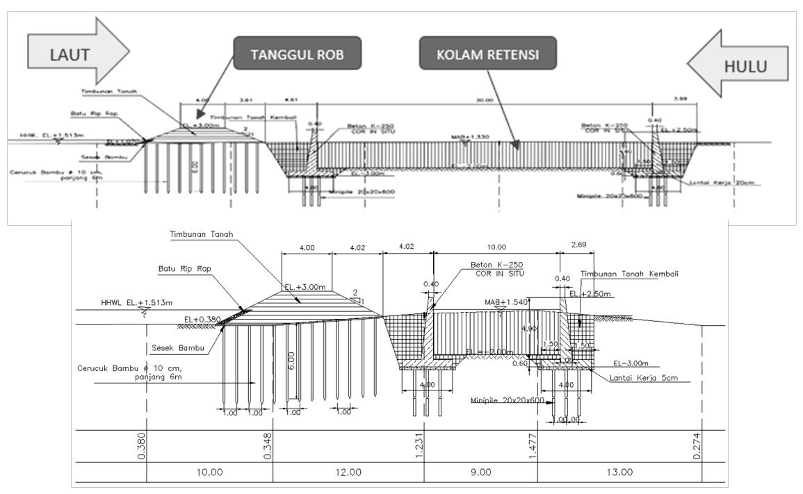
Figure 4. Design of coastal dike and retention ponds in the Sengkarang-Sragi Baru system (top) and the Bremi-Meduri system (bottom) [5] Source: Pemali Juana River Basin Organization
the Bremi-Meduri system. The average elevation of the coastal dike is + 3.00 - 3.40 m, and the average width of the coastal dike is ± 4.5 m.
Upstream of the coastal dike, a retention pond was built following the trace of the coastal dike. The retention pond in the Sengkarang-Sragi Baru system is 30 m wide. The retention pond in the Bremi-Meduri system is 10 m wide. The bottom elevation of the retention pond is -2.00 m, and the top elevation of the retention pond is +2.00 m, including the freeboard 0.5 m. The design of the coastal dike and retention pond can be seen in Figure 4.
There are two pump houses in the Sengkarang-Sragi Baru system. The first is the Silempeng pump house located west of the retention pond, which pumps water from the retention pond to the Silempeng River with two pumps, each with 2.0 m3 /s. Second, The Sengkarang pump houses, located at the east of the retention pond, pump water from the retention pond to the Sengkarang River with three pumps, each with 2.0 m3 /s. For the Bremi-Meduri system, there is one pump house, the Pabean pump house, located at the west of the retention pond, which functions to pump water from the retention pond downstream of the Meduri River with a total of two pumps, each with a capacity of 2 m3 /s. The pump will start operating when the water level in the retention pond is –0.5 m and stop working when the water level in the retention pond is –1.5 m. Currently, three pumps are added at the Mrican pump house, each with 2.0 m3 /s. With pump operating conditions like the others.
3. Data and Methodology
The stages of this research are literature study, data collection, data analysis, and conclusions. Topographic data in Digital Elevation Model (DEM) data was obtained from the Geospatial Information Agency (BIG) website. This data is used to analyze watershed parameters that are carried out using software-based Geospatial Information Systems (GIS). Field measurement data were obtained from the Pemali Juana River Basin Organization. Field measurement data in situational measurements, long section, river crosssection, coastal dike dimensions, and retention ponds are used as geometric inputs in hydraulics analysis.
Rainfall data were obtained from 5 stations around the study area, namely Wiradesa, Pekalongan, Pesantren Kletak, Kutosari/Doro, and Brondong stations. 19 years of rain data were used (2001-2019). This rain data is used as primary data in the hydrological analysis. The stages of hydrological analysis are regional rainfall analysis using Thiessen polygons, design rainfall analysis using frequency distribution analysis, hourly rainfall distribution using PSA 007 distribution, effective rainfall analysis using the SCS-CN method, design flood discharge analysis using Hydrologic Engineering Center-Hydrologic Modeling System (HEC-HMS) software based on SCS and Snyder Synthetic Unit Hydrograph method, and discharge calibration with observation discharge from the Pesantren Kletak weir.
Tidal data was obtained from the Pemali Juana River Basin Organization, carried out at the Sragi Baru River Estuary. Tidal data were analyzed using the Least Square method to determine the types of tides and the value of the tidal datum.
Hydraulics analysis using Hydrologic Engineering Center-River Analysis System (HEC-RAS) 1D with unsteady flow modeling. The upstream boundary used is the designed flood discharge of each river, and the downstream boundaries used are tidal elevation and Higher High-Water Level (HHWL) elevation.
Modeling scenario:
- · The conditions with coastal dike, retention ponds, Silempeng pumps, Sengkarang pumps, and Pabean pumps.
- · The conditions with the addition of 3 Mrican pumps, with a capacity of each pump 2 m3 /s.
- · The condition of adding 3 valve doors at Mrican with door dimensions of 2 x 2 m
4. Result
4.1. Topographical analysis
The topographic analysis is performed by processing Digital Elevation Model (DEM) data using GIS-based software to obtain watershed properties. This analysis produces 12 watersheds according to the river system in the study area, which can be seen in Figure 5 and Table 1.
Figure 5. Study area watershed map
The color in Figure 5 shows each watershed shown in Table 1 in order from left to right.
Table 1. Watershed parameters at the study area
| Watershed | Area (km2 ) | River Lenght (km) | ||||
|---|---|---|---|---|---|---|
| Sragi Baru | 362.167 | 68.235 | ||||
| Silempeng | 10.657 | 9.270 | ||||
| Semut | 1.151 | 2.246 | ||||
| Tratebang | 4.400 | 5.147 | ||||
| Mrican | 3.244 | 7.353 | ||||
| Pekuncen | 2.422 | 5.979 | ||||
| Pesanggrahan | 4.321 | 6.327 | ||||
| Sengkarang | 266.755 | 57.126 | ||||
| Meduri | 28.514 | 17.467 | ||||
| Bremi | 3.880 | 6.614 | ||||
| Drainase 1 | 3.837 | 5.102 | ||||
| Drainase 2 | 3.481 | 3.445 | ||||
4.2. Regional rainfall analysis
Analysis of regional rainfall using the Thiessen Polygon method from 5 (five) rainfall stations received from the rain data test. Thiessen polygon analysis using GIS software. The influence area of each rainfall post for each watershed in the study location is obtained. The results of the Thiessen polygon can be seen in Figure 6.
Figure 6. Thiessen Ppolygon area map in each watershed
The color in Figure 6 shows each watershed shown in Table 1 in order from left to right.
4.3. Design rainfall analysis
Design rainfall analysis uses frequency distribution analysis with Normal, Gumbel, Log-Normal, and Log Pearson III distributions (Chow, at al., 1998). Determination of the distribution used for each watershed in this study has been tested using the Chi-Square Test and Smirnov Kolmogorov Test (Triatmodjo, Bambang, 2008). The results of the analysis of the design rainfall after being multiplied by the Area Reduction Factor (ARF) in Table 2, following SNI 2415-2016, can be seen in Table 3.
4.4. Hourly rainfall distribution analysis
The analysis of the hourly rainfall distribution uses the PSA 007 distribution because there is no record of
Table 2. ARF values for each watershed
| Watershed | Area (km2 ) | ARF values |
|---|---|---|
| Sragi Baru | 362.167 | 0.84 |
| Silempeng | 10.657 | 0.97 |
| Semut | 1.151 | 0.99 |
| Tratebang | 4.400 | 0.99 |
| Mrican | 3.244 | 0.99 |
| Pekuncen | 2.422 | 0.99 |
| Pesanggrahan | 4.321 | 0.99 |
| Sengkarang | 266.755 | 0.85 |
| Meduri | 28.514 | 0.97 |
| Bremi | 3.88 | 0.99 |
| Drainase 1 | 3.837 | 0.99 |
| Drainase 2 | 3.481 | 0.99 |
| Sengkarang Kalibrasi (Pesantren Kletak Weir) | 239.040 | 0.86 |
Table 3. Design rainfall
| Design rainfall x ARF (mm) | ||||||||
|---|---|---|---|---|---|---|---|---|
| Return Period | 2 | 5 | 10 | 25 | 50 | 100 | 200 | 1000 |
| Sragi Baru | 105.913 | 122.416 | 131.042 | 140.242 | 146.184 | 151.529 | 156.422 | 166.508 |
| Silempeng | 112.514 | 134.619 | 146.174 | 158.496 | 166.456 | 173.615 | 180.168 | 193.679 |
| Semut | 112.514 | 134.619 | 146.174 | 158.496 | 166.456 | 173.615 | 180.168 | 193.679 |
| Tratebang | 112.514 | 134.619 | 146.174 | 158.496 | 166.456 | 173.615 | 180.168 | 193.679 |
| Mrican | 112.514 | 134.619 | 146.174 | 158.496 | 166.456 | 173.615 | 180.168 | 193.679 |
| Sengkarang | 117.624 | 153.199 | 171.795 | 191.626 | 204.436 | 215.959 | 226.504 | 248.248 |
| Pesanggrahan | 112.514 | 134.619 | 146.174 | 158.496 | 166.456 | 173.615 | 180.168 | 193.679 |
| Pekuncen | 112.514 | 134.619 | 146.174 | 158.496 | 166.456 | 173.615 | 180.168 | 193.679 |
| Meduri | 143.435 | 181.925 | 202.045 | 223.502 | 237.362 | 249.829 | 261.238 | 284.765 |
| Bremi | 146.392 | 185.676 | 206.211 | 228.11 | 242.256 | 254.98 | 266.625 | 290.636 |
| Drainase 1 | 146.392 | 185.676 | 206.211 | 228.11 | 242.256 | 254.98 | 266.625 | 290.636 |
| Dranase 2 | 146.392 | 185.676 | 206.211 | 228.11 | 242.256 | 254.98 | 266.625 | 290.636 |
| Outlet Pesantren Kletak Weir | 119.934 | 157.945 | 177.815 | 199.003 | 212.691 | 225.002 | 236.271 | 259.503 |
Table 4. Hourly rainfall for the 25-year return period
| Watershed | ||||||
|---|---|---|---|---|---|---|
| Time | Sragi Baru | Silempeng | Semut | Tratebang | Mrican | Sengkarang |
| 140.24 | 158.50 | 158.50 | 158.50 | 158.50 | 191.63 | |
| 0 | 0.00 | 0.00 | 0.00 | 0.00 | 0.00 | 0.00 |
| 1 | 2.80 | 3.17 | 3.17 | 3.17 | 3.17 | 3.83 |
| 2 | 2.80 | 3.17 | 3.17 | 3.17 | 3.17 | 3.83 |
| 3 | 4.21 | 4.75 | 4.75 | 4.75 | 4.75 | 5.75 |
| 4 | 7.01 | 7.92 | 7.92 | 7.92 | 7.92 | 9.58 |
| 5 | 12.62 | 14.26 | 14.26 | 14.26 | 14.26 | 17.25 |
| 6 | 63.11 | 71.32 | 71.32 | 71.32 | 71.32 | 86.23 |
| 7 | 21.04 | 23.77 | 23.77 | 23.77 | 23.77 | 28.74 |
| 8 | 9.82 | 11.09 | 11.09 | 11.09 | 11.09 | 13.41 |
| 9 | 7.01 | 7.92 | 7.92 | 7.92 | 7.92 | 9.58 |
| 10 | 4.21 | 4.75 | 4.75 | 4.75 | 4.75 | 5.75 |
| 11 | 4.21 | 4.75 | 4.75 | 4.75 | 4.75 | 5.75 |
| 12 | 1.40 | 1.58 | 1.58 | 1.58 | 1.58 | 1.92 |
| Watershed | ||||||
|---|---|---|---|---|---|---|
| Time | Pesanggrahan | Pekuncen | Meduri | Bremi | Drainase 1 | Dranase 2 |
| 158.50 | 158.50 | 223.52 | 228.11 | 228.13 | 228.13 | |
| 0 | 0.00 | 0.00 | 0.00 | 0.00 | 0.00 | 0.00 |
| 1 | 3.17 | 3.17 | 4.47 | 4.56 | 4.56 | 4.56 |
| 2 | 3.17 | 3.17 | 4.47 | 4.56 | 4.56 | 4.56 |
| 3 | 4.75 | 4.75 | 6.71 | 6.84 | 6.84 | 6.84 |
| 4 | 7.92 | 7.92 | 11.18 | 11.41 | 11.41 | 11.41 |
| 5 | 14.26 | 14.26 | 20.12 | 20.53 | 20.53 | 20.53 |
| 6 | 71.32 | 71.32 | 100.58 | 102.65 | 102.66 | 102.66 |
| 7 | 23.77 | 23.77 | 33.53 | 34.22 | 34.22 | 34.22 |
| 8 | 11.09 | 11.09 | 15.65 | 15.97 | 15.97 | 15.97 |
| 9 | 7.92 | 7.92 | 11.18 | 11.41 | 11.41 | 11.41 |
| 10 | 4.75 | 4.75 | 6.71 | 6.84 | 6.84 | 6.84 |
| 11 | 4.75 | 4.75 | 6.71 | 6.84 | 6.84 | 6.84 |
| 12 | 1.58 | 1.58 | 2.24 | 2.28 | 2.28 | 2.28 |
hourly rainfall in the study area, according to the Technical Instructions for Calculation of Flood Discharge in Dams (Triatmodjo, Bambang, 2008). The duration of the rainfall used is 12 hours. Hourly rainfall for the 25-year return period is shown in Table 4. The 25-year return period is used by the Regulation of the
Minister of Public Works and Housing Number 28/ PRT/M/2015 and the document Pola Water Resource Management in the Pemali Comal River Area.
4.5. Effective rainfall analysis
Analysis of effective rainfall uses the SCS method with a Curve Number (CN) value. The CN value was obtained from land cover data from the Ministry of Environment and Forestry with a soil type map of the Harmonized World Soil Database (HSDW). The CN value is input in the HEC-HMS software in flood discharge analysis design. The CN values for each watershed can be seen in Table 5.
4.6. Design Flood discharge analysis
Design flood discharge analysis using the HEC-HMS software with the Synthetic Unit Hydrograph SCS and Snyder methods. The inputs from this modeling are watershed parameters, river systems, hourly distribution of rainfall, and CN values to calculate
Table 5. Curve number value for each watershed in the study area
| Watershed | Composite CN Value |
|---|---|
| Sragi Baru | 68.66 |
| Silempeng | 72.44 |
| Semut | 71.77 |
| Tratebang | 74.19 |
| Mrican | 84.57 |
| Pekuncen | 77.89 |
| Pesanggrahan | 80.79 |
| Sengkarang | 61.95 |
| Meduri | 73.77 |
| Bremi | 75.51 |
| Drainase 1 | 81.15 |
| Drainase 2 | 74.99 |
infiltration. The modeling was carried out at the outlet of the Kletak Pesantren Weir for calibration purposes. After being calibrated, the modeling is carried out for the study area. The HEC-HMS model for the study site can be seen in Figure 7.
Calibration compares the peak discharge from the design flood discharge with the peak discharge from observations at the Pesantren Kletak Weir. Synthetic Unit Hydrograph SCS was selected from the calibration results with a value of Ct = 1, which would then be used for analysis at the study site. The results of the calibration are shown in Figure 8.
Based on the Synthetic Unit Hydrograph SCS analysis, the peak flood discharge for the 25-year return period is shown in Figure 9 and Table 6.
4.7. Tidal analysis
Based on the tidal analysis results using the Least Square method, the Formzhal number value is 0.53 (mixed semi-diurnal), and the HHWL value is 1.16 m.
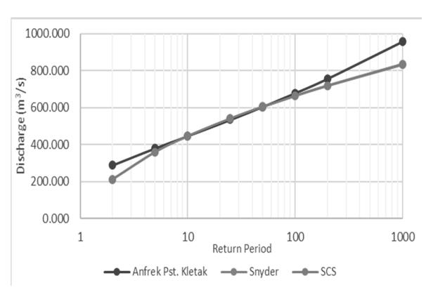
Figure 8. The results of the calibration of the discharge at the Pesantren Kletak Weir outlet
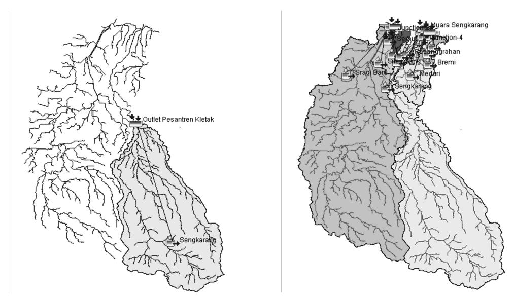
Figure 7. HEC-HMS modeling setup at the Pesantren Kletak Weir outlet (left) HEC-HMS modeling setup at the study area (right)
The color in Figure 7 (right) shows each watershed shown in Table 1 in order from left to right.
144 Jurnal Teknik Sipil
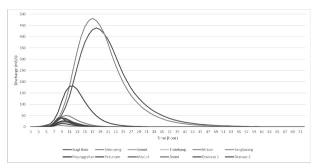
Figure 9. SUH SCS return period of 25 years for each watershed
Table 6. Recapitulation of the maximum discharge of each watershed
| Watershed | 25 -year return period (m3 /s) |
|---|---|
| Sragi Baru | 439.10 |
| Silempeng | 50.90 |
| Semut | 7.00 |
| Tratebang | 24.80 |
| Mrican | 20.60 |
| Sengkarang | 481.40 |
| Pesanggrahan | 26.00 |
| Pekuncen | 14.30 |
| Meduri | 181.40 |
| Bremi | 39.50 |
| Drainase 1 | 40.10 |
| Drainase 2 | 39.30 |
4.8. Hydraulics analysis
Modeling for hydraulic analysis using HEC-RAS 1D software with the unsteady flow. Modeling is carried out under the following conditions:
a. The conditions with coastal dike, retention ponds, Silempeng pumps, Sengkarang pumps, and Pabean pumps.
· Sengkarang - Sragi Baru System
The concept of this condition is to close the Semut, Tratebang, Mrican, Pekuncen, Pesanggrahan rivers with coastal dike. In the model, an inline structure is made for a coastal dike with a peak elevation of + 3.40 m and a storage area to model a retention pond with 4,955 m2 wide, the minimum elevation of the retention pond – 2.00 m. Modeling of the Silempeng Pump (2 x 2 m3 /s), which pumps water from the retention pond to the Silempeng River, and the Sengkarang Pump (3 x 2 m3 /s), which pumps water from the retention pond to the Sengkarang River, the pump starts at water elevation – 0.50 m and off at an elevation of – 1.50 m. The setup model on HEC-RAS for the Sengkarang-Sragi Baru system can be seen in Figure 10.
The results of the modeling can be seen in Figure 11.
Figure 11 shows the peak condition when a Q25 flood on the Mrican River. There is still flooding in the upstream area. This condition is due to the limited capacity of the retention pond and the existing pump capacity. The pump will periodically lower the flood
Figure 10. Modeling with coastal dike, retention ponds, Silempeng and Sengkarang pumps
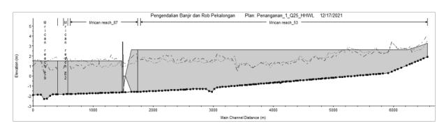
Figure 11. The peak condition of the 25-year return period flood on the Mrican River
elevation up to the target of the water elevation. The target of this polder system is to lower the water to an elevation of – 1.50 m. To pump up to an elevation of – 1.50 m, the Silempeng Pump operates for 150 hours and the Sengkarang Pump for 150 hours. The relation between pump operating time and water level conditions can be seen in the figure below.
· Bremi - Meduri System
The concept of this condition is to cover environmental drainages with a coastal dike. In the model, an inline
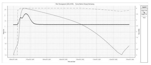
Figure 12. Graph of the relation between Silempeng pump operation and retention pond water level
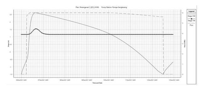
Figure 13. Graph of the relation between Sengkarang pump operation and retention pond water level
structure is made for the coastal dike with a peak elevation of + 3.40 m and a storage area to model the retention pond with a 2,311 m2 wide, the minimum elevation of the retention pond – 2.00 m. Modeling the Pabean Pump (2 x 2 m3 /s) pumping water from the retention pond to the Meduri River, the pump starts at a water elevation of – 0.50 m and turns off at an elevation of – 1.50 m. The setup model on the HEC-RAS for the Bremi-Meduri system can be seen in Figure 14. The results of the modeling can be seen in Figure 15.
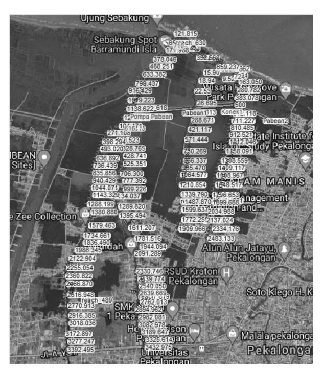
Figure 14. Modeling with coastal dike, retention ponds, and Pabean pump
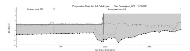
Figure 15. Flood conditions 25-year return period on the Bremi-Meduri system
From the modeling results, to achieve the target water level elevation at an elevation of – 1.50 m, the Pabean Pump operational time is 72 hours. The relation between pump operating time and water level conditions can be seen in Figure 16.
b. Conditions with the addition of 3 Mrican pumps, with a capacity of each pump 2 m3 /s.
In the Sengkarang-Sragi Baru system, the Mrican Pump model (3 x 2 m3 /s) is added, which pumps water from the retention pond to the Mrican River. The pump starts at a water elevation of – 0.50 m and turns off at an elevation of – 1.50 m. The setup model on the HEC -RAS can be seen in Figure 17.
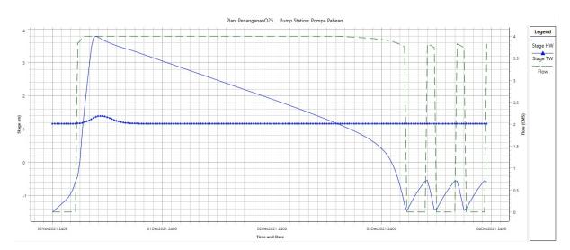
Figure 16. Graph of the relation between Pabean pump operation and retention pond water level
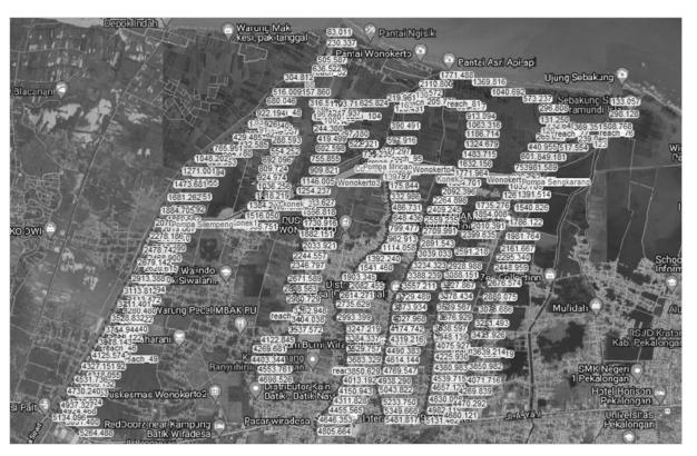
Figure 17. Modeling the addition of a Mrican pump to the Sengkarang-Sragi Baru system
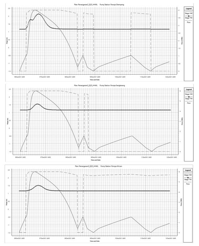
Figure 18. (a) The graph of the relation between the operation of the Silempeng pump and the water level elevation of the retention pond after the addition of the Mrican pump; (b) The graph of the relation between the operation of the Sengkarang pump and the water level elevation of the retention pond after the addition of the Mrican pump; © The graph of the relation between the operation of the Mrican pump and the water level elevation of the retention pond
With the addition of the Mrican pump to pump floods up to an elevation of – 1.50 m, it takes 49 hours for the Silempeng Pump, 49 hours for the Sengkarang Pump, and 49 hours for the Mrican Pump. The relation between pump operating time and water level conditions can be seen in the Figure 18.
c. The condition of adding 3 valve doors at Mrican with door dimensions of 2 x 2 m
The location of the valve door is on a coastal dike that closes the Mrican River channel. When the water elevation in the retention pond is higher than sea level, the valve door will open, and water from the retention pond will flow out through the valve door into the Mrican River so that the downstream boundary used is the tidal elevation of seawater.
With the valve door at Mrican, to pump floods up to an elevation of – 1.50 m, it takes 36 hours for the Silempeng Pump, 36 hours for the Sengkarang Pump, and 36 hours for the Mrican Pump. The relation between pump operating time and water level conditions can be seen in the figure below.
5. Conclusions
From the results of this study, it can be concluded that:
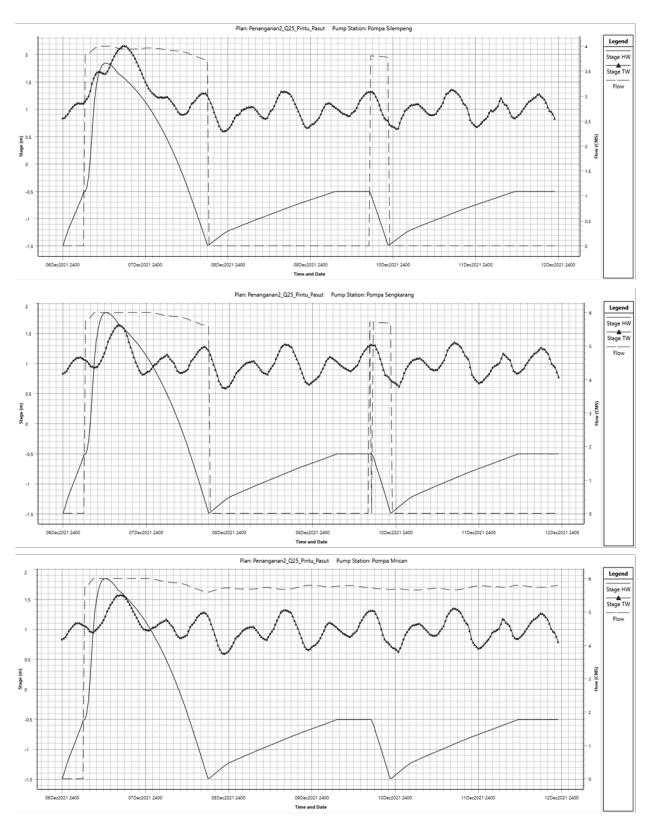
Figure 19. (a) The graph of the relation between the operation of the Silempeng pump and the water level elevation of the retention pond after the addition of the Mrican valve door; (b) The graph of the relation between the operation of the Sengkarang pump and the water level elevation of the retention pond after the addition of the Mrican valve door; (c) The graph of the relation between the operation of the Mrican pump and the water level elevation of the retention pond after the addition of the Mrican valve door
- 1. In the Sengkarang-Sragi Baru System, to pump the 25-year return period flood up to a water level of – 1.50 m, it takes 150 hours for the Silempeng Pump and 150 hours for the Sengkarang Pump.
- 2. In the Bremi-Meduri System, to pump the 25-year return period flood up to water level – 1.50 m, the Pabean Pump operational time is 72 hours.
- 3. In the Sengkarang-Sragi Baru System, after the addition of the Mrican Pump to pump the 25-year return period flood up to a water elevation of – 1.50 m, the Silempeng Pump operational time is 49 hours, the Sengkarang Pump is 49 hours, and the Mrican Pump is 49 hours. This shows that the addition of the Mrican Pump has succeeded in reducing the operating time of the pump to reduce flooding in the Sengkarang-Sragi Baru System for 101 hours.
- 4. With the addition of the Flap gate at Mrican, it takes 36 hours for the Silempeng Pump, 36 hours for the Sengkarang Pump, and 36 hours for the Mrican Pump. This shows that the addition of a flap gate at Mrican has succeeded in reducing the operating time of the pump to reduce flooding in the Sengkarang-Sragi Baru System for 13 hours. So The addition of Mrican pumps and flap gates can reduce pump operating time to support the success of Coastal Dike and Retention Ponds in controlling floods and tidal in Pekalongan.