
Abstrak
Studi mengenai persepsi masyarakat terhadap jalan tol selama periode ramp-up masih jarang dilakukan, hal ini penting untuk menilai kelayakan investasinya. Makalah ini bertujuan untuk menetapkan pendekatan pertama dalam memodelkan persepsi individu pelaku perjalanan komuter selama periode tersebut sebagai proses belajar dan beradaptasi terhadap jalan tol yang baru beroperasi. Khususnya, upaya untuk mengidentifikasi sikap dan perilaku individu pelaku perjalanan terhadap jalan tol antar kota penghubung kawasan aglomerasi yang sedang berkembang. Pengumpulan data dilakukan melalui survei revealed dan stated preference dengan teknik bola salju (snowball sampling) yang menggunakan media sosial. Kemudian kami mengembangkan model logit-biner untuk mengeksplorasi persepsi penumpang komuter terhadap jalan tol pada periode ramp-up dan hasilnya menunjukkan bahwa ketika melakukan aktivitas perjalanan, pelaku perjalanan komuter lebih memilih menggunakan jalan tol dengan atribut yang paling berpengaruh terhadap pengambilan keputusan masing-masing adalah, waktu tempuh, biaya perjalanan, jarak gerbang tol, jarak tempuh, umur penumpang, keindahan pemandangan dan frekuensi penggunaan jalan tol. Makalah ini juga menunjukkan bahwa preferensi positif terhadap jalan tol pada periode ramp-up tidak selalu terkait dengan kemacetan lalu lintas seperti di wilayah perkotaan yang padat, keberadaan lalu lintas tamasya sangat potensial mempengaruhi.
Kata-kata kunci: Perilaku pemilihan rute, model logit-biner, jalan tol, periode ramp-up
1. Introduction
Toll road infrastructure is still believed to be the artery of equitable development in developing countries. Indonesia, for example, which has included toll road
infrastructure development in the list of national strategic projects (PSN) as its priority scale. However, in its implementation, the construction of toll roads in Indonesia is always faced with funding problems. The funding mechanism with the public-private partnerships
(PPP) scheme has been implemented, but it has not encouraged domestic and foreign investors to get involved, this is related to the high investment risk that will be faced. According to the World Bank, traffic risk is an unavoidable risk in toll road investment, given our imperfect ability to predict traffic and revenue a long way (often several decades) into the future. Thus, traffic forecasts are employed in the toll road sector to gauge the bankability of candidate investment projects by private sector investors. Banks (or other investors) are commonly most sensitive to early year asset performance as a project's cumulative cash flow curve will be at its lowest point. All of the project debt has been drawn down yet project revenues are only just starting to be generated. The potential for project distress (and possibly default on debt repayments) is arguably at its greatest during the earliest years of project operations (Bain, 2009). In fact, the results of studies on Toll road traffic forecasting performance tend to be overestimated by 20% to 30% in the first few years after operation (Bain and Wilkins, 2002; Flyvbjerg, at al., 2006). The phenomenon is referred to as a ramp-up period which is a short-term acute problem in transportation infrastructure investment (Transport Research Board, 2006).
The ramp-up period associated with certain learning and adaptation of the regional travelers to the new travel conditions created by new toll roads etc. The learning and adaptation process will affect changes in the travel behavior pattern of each individual traveler as a psychological effect (Perez, at al., 2012). McFadden (McFadden, 2007) stated that cognitive psychological effects will affect the traveler's decision-making attitude during the route choice process. Travelers need time to know and feel the benefits that will be received (such as saving time or travel costs, travel comfort, safety, etc.) when using the toll road segment. Thus, there may be delays in building potential user demand for newly operating toll roads (Douglas, 2003; Chang, at al., 2010). The conventional model that is generally used has not been able to predict traffic during that period (Chang, at al., 2010; Hartgen, 2013), because the potential traffic demand during the ramp-up period tends to be influenced by the travel behavior of each of the travelers so it would be more appropriate to use a disaggregation model (Núñez, 2008).
The paper aims to establish a first approach in modeling the perceptions of individual commuter travelers during the learning process and adaptation to newly operating toll roads (in other words during the ramp-up period). Particularly, efforts to identify the attitudes and behaviors of individual commuter travelers towards interurban toll roads that connect between developing agglomeration areas. Thus, it can help the government, transportation agencies, traffic consultants, investment bankers, investors and other related institutions in making the appropriate decisions.
2. Literature Review
Previous toll road studies related to ramp-up periods mostly focused on assessing the performance between traffic forecasts and actual conditions (Flyvbjerg, 2005; Odeck and Welde, 2017 ). By contrary, literature related to the perceptions of travelers on toll roads during the period are still not widely found, although there are some who have examined attitudes towards toll roads from another perspective (Podgorski and Kockelman, 2006; Burris, at al., 2004). In addition to helping to analyze and understand the behavior of travelers, route choice models are also used to model traffic assignments in transportation planning, forecasting traffic flows, designing new transportation infrastructure and investigating new policies (Prato, 2009; Alizadeh, at al., 2019). Therefore, understanding the traveler's route choice behaviors and the factors that influence it is of utmost importance.
When new toll roads open, changes to regional travel patterns will occur. Travelers, in the process of utility maximization and cost minimization of their travel activities when using the newest alternative route of toll roads, are understood to develop their final decisions by learning from their mistakes (Chang, 2010). The adjustment to trip patterns is due to users' lack of understanding of the new toll road and the benefits (Núñez, 2008). During this event, the demand for toll roads will continue to increase and the curve tends to fluctuate. However, over time, the oscillations will lessen until they reach the steady state phase (D'Este, 2010). The period of time it takes to stabilise or steady state is called the duration of the ramp-up (Li and Hensher, 2010).
According to Bogers, Bierlaire, and Hoogendoorn (Bogers, at al., 2007), there are two types of learning found in psychological learning theory appear to play a role in day-to-day route choice: implicit (reinforcement -based) and explicit (belief-based). Implicit learning, also known as operant conditioning, comprises all kinds of learning in which repetition of the relationship between stimulus and response patterns leads to a mental representation (memory). Whereas explicit learning relates to the effect of travel information on route choice, because the information itself does not give any reinforcement but does allow for constructing new knowledge about the routes. Habit is another phenomenon that causes people to choose without rationally weighing all the available alternatives and their respective strengths and weaknesses each time a decision needs to be made (Bogers, at al., 2005).
Performing the same trip many times (such as a commuter trip), travelers can learn about available routes from their experiences (Bogers, at al., 2005) based on a repetitive decision process (Wei, at al., 2014). But in fact, in the real world drivers don't always choose the route with the least costly routes (Zhu and Levinson, 2015), due to lack of information and behavioral inertia, or other reasons (Shang, at al., 2017). It is hard for travelers to make the best choices every time because of their bounded rationality and environmental uncertainty. Therefore, route choice behavior follows stochastic rules or dynamic behavior response (Wei, at al., 2014; Di and Liu, 2016). The results of a laboratory-scale study by Knorr, Chmura, and Schreckenberg (Knorr, at al., 2014) regarding the choice between high-capacity toll roads and toll-free
main roads, stated that travelers improve their decisions over time as a result of learning, even though there is no a stable equilibrium point (Wardrop's User Equilibrium). For new travelers, learning about route attributes is considered important in the first few days of travel adjustment, but over time the information provided and the habit factors developed will become more important (Bogers, at al., 2005; Khoo and Asitha, 2016). According to Moghaddam et al. (Moghaddam, at al., 2019), some important determinants of route choice and adjustment to available information, respectively, were the purpose of the trip, the reliability of travel time, and income.
According to Jan, Horowitz, and Peng (Jan, at al., 2000), factors affecting route choice decisions can be classified into four categories of observable variables including travelers' attributes (such as age, gender, ducation, income, etc.), route attributes (such as traffic conditions, speed limits, number of turns, pavement quality, etc.), trip attributes (such as trip purpose, travel time, etc.), and circumstances (such as weather conditions, time of day, traffic information, etc.). However, choice decisions might not be exclusively dependent on these observable variables, but also on latent variables, which cannot be directly observed, and measured, such as attitudes, norms, perceptions, lifestyle and beliefs (Alizadeh, at al., 2019). Prato, Bekhor, and Pronello (Prato, at al., 2012 provided insight into the comprehension of the determinants of route choice behavior by proposing and estimating a hybrid model that integrates latent variable and route choice models. The model is a measurement equation that describes the relationship between utility indicators and latent variables from available route alternatives, as well as structural equations of observable characteristics with latent variables or utility with explanatory variables from available alternative routes. By considering latent variables (i.e., memory, habits, familiarity, spatial ability, time saving skills) in addition to traditional variables (for example, travel time, distance, and congestion level), the model estimate will result in an illustration that the traveler behavior route choice will be better.
Random utility discrete choice models are among the most frequently used approaches to model, analyze and understand these behaviors (Prato, 2009; Dhakar and Srinivasan, 2014). Gomez, Papanikolaou, and Vassallo (Gomez, at al., 2017) have developed both a binomial logit and a censored regression (tobit) model to explore drivers' perceptions and willingness to pay in interurban toll roads in Spain. The results showed that toll road users who come from areas with a more extensive tolled network generally have a negative attitude towards costs, but they don't necessarily have lower willingness to pay. In addition, the asymmetrical distribution of toll roads between regions will have an impact on negative perceptions among users who feel they are being treated unfairly. The literature has shown that the road usage patterns are dynamic: drivers interact with each other, they evaluate their travel expenses and adapt their behavior. This might be the reason for the clear differences between stated preference (i.e., response to hypothetical choices) and revealed preference (i.e., response to actual choices) studies in the literature (Knorr, at al., 2014; Brownstone and Small, 2005).
3. Methodology
To achieve the goal of this study, the influence of Soreang toll road infrastructure on the commuter travel behavior in the greater Bandung area during the rampup period was investigated. First, a survey containing travelers' Revealed Preference (RP) and Stated Preference (SP) was conducted to obtain the travelers' characteristics, their actual and preferred travel route choice. Second, determine the factors that explain the relationship or correlation between the independent variables as observational variables from the survey data attributes and then reduce them as a whole into several explanatory components that influence route choice decisions making of individual commuter travelers by the principal component analysis (PCA) method. Then, the preference characteristics are measured based on the utility maximization theory and choice behavior theory. Afterward, the parsimonious model constructed using the stepwise method was proposed. Finally, the predictive accuracy of the proposed model is validated by statistical analysis.
3.1 Travel data collection
The Soreang-Pasirkoja (abbreviated as Soroja) toll road which has a length of 10.55 km functions as an accessibility for the agglomeration area between Bandung City, Cimahi City and Soreang which is the capital and government center of Bandung Regency, West Java in Indonesia. The travel time from Bandung to Soreang can be shortened by using this toll road, which was originally about 2 hours away via Jalan Kopo to an average of 12 minutes. The purpose of its construction is to attract interest of tourists to visit tourist attractions in the Bandung Regency or Southern Bandung area, which previously was only centered in the Bandung City or the North Bandung area. The Soreang toll road is part of the greater Bandung transportation network which is connected to the Padalarang-Cileunyi (abbreviated as Padaleunyi) toll road.
The geographic location of the Soroja toll road network is shown in Figure 1. The toll road which was opened since December 2017, the average traffic volume passing through the Soreang toll gate on weekends is 35,379 vehicles per day, but different on weekdays
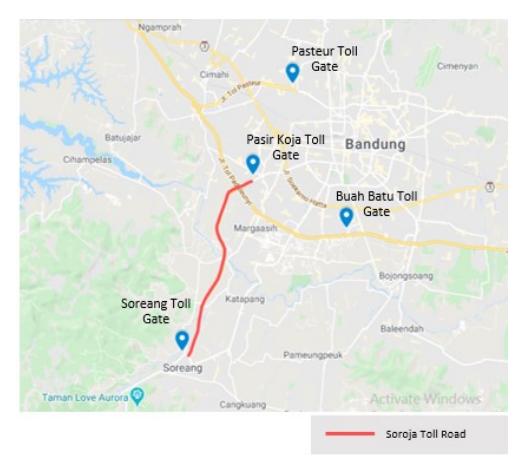
Figure 1. The network of Soroja toll road.
around 20000 vehicles per day. The decrease in traffic volume on weekdays is due to the potential for toll road users, generally commuter travelers, who are regional movements of the agglomeration areas of Bandung City, Cimahi City and Soreang.
The data collection was aiming to measure the perceptions of regional commuter travelers as potential users of the Soroja toll road in the agglomeration area, namely Bandung City, Cimahi City and Soreang. Respondents in this study were civil servants, private employees, students or other. They were commuter travelers whose travel activities by car and route selection involve the Soroja toll road. The online-based questionnaire was conducted using a snowball sampling technique using social media, such as WhatsApp, Facebook, etc. Snowball sampling is undertaken when a qualified participant shares an invitation with other subjects similar to them who fulfill the qualifications defined for the targeted population. The survey questionnaire was designed to identify the factors that influence respondents' behavior and attitudes in route choice, including traveler attributes (such as age, gender, education, occupation, monthly income, household size, and number of car ownership in the household), trip attributes (such as origin-destination trip, trip purpose, frequency of using toll roads, departure time, etc.) and route attributes (such as travel time, travel costs, distance of toll gate, travel distance, safety, speed limits, traffic conditions, scenic, pavement quality, and number of traffic light intersections, toll tariff rate). The RP and SP surveys collected the information of respondents' preferred route based on the evaluation process of learning and adaptation to the aforementioned factors during the ramp-up period. The RP and SP surveys collected the information of the respondents' preferred route to the Soroja toll road during the ramp-up period, because the service period was still around two years (Bain and Wilkins 2002; Li and Hensher 2010). The detailed survey information is shown in Table 1.
3.2 Binary logit models to measure users' perceptions
A binary logit model was applied in this study to analyze the effect of socio-economic and demographic factors, trip attributes and route attributes to the attitudes and behavior of commuter travelers as potential toll road users. The model approach is based on the principle of utility maximization. Rationally, an individual traveler selects alternative choice set offered (e.g. using toll roads or non-toll roads when traveling) with the highest utility value (Gomez, at al., 2017). In this study, respondents were asked in the survey whether they considered the toll road as the appropriate route for their travel activities. This answer represented the dependent variable of the binary choice specification which has only zero and one values. This can be expressed mathematically as in Equation (1).
If \[U_{ir}(X_{ir}, S_i)\] \(^3U_{ik}(X_{ik}, S_i)\) "\(k \triangleright r \square k\), "\(k \hat{1} C_i\) (1)
Where \(U_{ir}\) (), \(U_{ik}\) () are the utility functions of alternatives r and k for individual i; \(X_{ir}\) and \(X_{ik}\) are vectors of attributes describing alternatives r and k for individual i (e.g., travel time, travel cost, and other relevant attributes of the available routes); \(S_i\) is a vector of characteristics describing individual i, that influence his/her preferences among alternatives (e.g., household income and number of automobiles owned for travel route choice); r > k means the alternative to the left is preferred to the alternative to the right; and "k is for all cases, k, in the choice set alternatives.
Equation (1) can be interpreted, if the utility of alternative r is greater than or equal to the utility of all alternatives k, alternative r will be preferred and chosen from the set of alternatives \(C_i\). In fact, individual travelers may not have information or misperceptions about the attributes of some or all of the alternatives. As a result, different individuals, each with different information or perceptions about the same alternatives are likely to make different choices. Thus, random utility models or probability choice are more appropriate, especially when individual travelers are still learning and adaptation to new alternatives. The random utility equation is given by (Hensher, at al., 2015):
\[U_{ir} = V_{ir} + \mathcal{E}_{ir} \tag{2}\]
Where \(V_{ir}\) is a measurable component (deterministic) or a systematic component of alternative utility r for individual i; and \(\varepsilon_{ir}\) is a residual value of random error or utility unknown or a disturbance term of alternative r for individual traveler i. Usually, the systematic component is a linear function of the parameter as the following Equation (Hensher, at al., 2015; Xu, at al., 2014):
\[V_{ir} = \sum_{t=0}^{T} \beta_{tr} x_{tir} \tag{3}\]
The utility function for individual traveler i and alternative r in Equation (3) are detailed as Equation (4) as follows:
\[V_{ir} = \beta_0 + \beta_{1r} x_{1ir} + \beta_{2r} x_{2ir} + \beta_{3r} x_{3ir} + \dots + \beta_{Tr} x_{Tir}\] (4)
Table 1. The description of the SP and RP survey.
| Surveys | Information to collect | Description |
|---|---|---|
| RP survey | Socio-economic (personal attributes) | Age, gender, education, occupation, income, Household size, household car number |
| RP survey | Travel information last time when using toll roads and non-toll roads (other contributing factors) | Travel time, travel cost, toll gate distance, travel speed, travel distance, traffic congestion, scenic beauty, traffic light, land use along the road, road condition, departure time and the frequency of using toll road |
| SP survey | Preferred route choice under travel scenarios | Hypothetic travel time, travel cost (toll tariff rate), toll gate distance, travel distance |
342 Jurnal Teknik Sipil
Table 2. Description of variables.
| Type | Variable | Description |
|---|---|---|
| Dependent | Using toll versus non-toll road | |
| variable | ROUTE_CHOICE | 1 – toll road, 2 – non-toll road |
| Independent | Attributes in route choice | |
| variable | TRAVEL_TIME | Perceived total time from origin (e.g. home) to destination (e.g. office) using Toll and Non Toll Road (in minutes) |
| TRAVEL_COST | Perceived total cost from origin (e.g. home) to destination (e.g. office) using Toll and Non Toll Road (in Indonesian Rupiah) | |
| TOLL_GATE | Distance from origin (e.g. home) to toll gate | |
| Less than 0,5 km | Indicator for at Less than 0,5 km | |
| 0,6 – 1,5 km | Indicator for 0,6 – 1,5 km | |
| 1,6 – 2,5 km | Indicator for 1,6 – 2,5 km | |
| 2,6 – 3,5 km | Indicator for 2,6 – 3,5 km | |
| More than 3,5 km | Indicator for more than 3,5 km | |
| TRAVEL_SPEED | Maximizing travel speed 1 – strongly disagree, 2 – disagree, 3 – neutral., 4 – agree, 5 – strongly agree | |
| TRAVEL_DISTANCE | (abbreviated below) Distance to travel destination | |
| Less than 1,5 km | Indicator for at Less than 1,5 km | |
| 1,6 – 4,5 km | Indicator for 1,6 – 4,5 km | |
| 4,6 – 7,5 km | Indicator for 4,6 – 7,5 km | |
| 7,6 – 10,5 km | Indicator for 7,6 – 10,5 km | |
| More than 10,5 km | Indicator for more than 10,5 km | |
| TRAFFIC_CONG | Avoiding traffic congestion 1 – strongly disagree, 2 – disagree, 3 – neutral., 4 – agree, 5 – strongly agree (abbreviated below) | |
| TRIP_PUR | Depending on the level of importance of trip purpose 1 – str. disag, 2 – disag., 3 – neu., 4 – ag., 5 – str. ag | |
| SCENIC_BEAUTY | Preferring scenic routes | |
| TRAFFIC_LIGHT | 1 – str. disag, 2 – disag., 3 – neu., 4 – ag., 5 – str. ag Avoiding traffic lights of road intersection | |
| HIST_ACC | 1 – str. disag, 2 – disag., 3 – neu., 4 – ag., 5 – str. ag Avoiding routes with high accident events | |
| DROP_OFF | 1 – str. disag, 2 – disag., 3 – neu., 4 – ag., 5 – str. ag Preferring route that can stop anywhere | |
| LU_ROUTE | 1 – str. disag, 2 – disag., 3 – neu., 4 – ag., 5 – str. ag Much activities along the road, such as shops or offices | |
| ROAD_COND | 1 – str. disag, 2 – disag., 3 – neu., 4 – ag., 5 – str. ag Importance of pavement quality | |
| Demographic | Socio-economic attributes | 1 – str. disag, 2 – disag., 3 – neu., 4 – ag., 5 – str. ag |
| Variables | INCOME | Monthly household income (IDR) |
| Less than 3.000 thousand IDR | Indicator for at Less than 3.000 thousand IDR | |
| 3.000 to 7.000 thousand IDR | Indicator for 3.000 to 7.000 thousand IDR | |
| 7.001 to 10.000 thousand IDR | Indicator for 7.001 to 10.000 thousand IDR | |
| More than 10.000 thousand IDR GENDER | Indicator for more than 10.000 thousand IDR Indicator for gender | |
| 1 – Male, 0 – Female | ||
| AGE | Years old | |
| Young (17 to 39) | Indicator for 17 to 39 years old | |
| Middle age (40 to 59) | Indicator for 40 to 59 years old | |
| Travel | Old (more than 60) Travel on Toll Roads | Indicator for more than 60 years old |
| variable | FREQ | Frequency of use of toll roads by commuter traveler |
| More than four times a week | Indicator for more than 4 days a week | |
| At least once a week | Indicator for at least once a week | |
| At least once a month | Indicator for at least once a month | |
| At least once a year | Indicator for at least once a year | |
| Less than once a year DEPARTURE TIME | Indicator for at Less than once a year | |
| (Western Indonesian Time) 06.00 - 09.00 | Routine departure time of travel activities Indicator for departure time at 06.00 - 09.00 | |
| 11.00 - 14.00 | Indicator for departure time at 11.00 - 14.00 | |
| 16.00 - 19.00 | Indicator for departure time at 16.00 - 19.00 | |
| 21.00 - 24.00 | Indicator for departure time at 21.00 - 24.00 |
where \(b_0\) is known as an alternative specific constant (ASC), describing something of the alternative utility unrelated to the attribute specified in the utility function, \(b_{tr}\) is the vector of unknown parameters to be estimated and assumed to be constant for all individuals in the homogeneous set (fixed coefficients model) but vary across to attribute t for alternative r; and \(x_{tir}\) is the vector of attributes t of alternative r for individual traveler t. The utility function for traveler t, alternative t is expressed as Equation (4). The variables used in the utility function in this study are shown in Table 2.
If the random component of \(\varepsilon\) is independent and identically distributed (IID) and follow the Gumbel distribution, then probability formula of alternative r is chosen by individual i can be write down as follows:
\[P_{i}(r) = \frac{e^{V_{ir}}}{\sum_{k \in C} e^{V_{ik}}}\] (5)
Where \(P_i(r)\) is the probability of alternative r is chosen by individual i (the magnitude of the probability \(P_i(r)\)
is \[0 \, {\mathfrak t} \, P_i(r) \, {\mathfrak t} \, 1\], for all \(i \, \hat{1} \, C_i\) and \(\sum_{i \in C_i} P_i(r) = 1\)). The odds
ratio represents the odds of an outcome occurring based on some known probability. The odds of an outcome occurring may be calculated as per Equation (6):
\[Odds(Y) = \frac{P_i(r)}{1 - P_i(r)} \tag{6}\]
For the logit model, the link function used is the log-odds. Algebraically the logit probabilities for the binary outcome case can be derived as per Equation (7):
\[\ln\left(\frac{P_{i}(r)}{1 - P_{i}(r)}\right) = \beta_{0} + \beta_{1r}x_{1ir} + \beta_{2r}x_{2ir} + \beta_{3r}x_{3ir} + \dots + \beta_{Tr}x_{Tir} \quad (7)\]
The goal of logistic regression is to estimate the T+1 unknown parameters b in Equation (3). This is done with maximum likelihood (ML) estimation which entails finding the set of parameters for which the probability of the observed data is greatest. The ML equation is derived from the probability distribution of the dependent variable (the log-odds) by estimating the parameter values that are most likely to occur in the observed sample.
The results of the logistic regression process can be interpreted into three different levels. First, each term in the equation represents contributions to estimate the log-odds. Thus, for each one unit increase (decrease) in \(x_{tir}\), there is predicted to be an increase (decrease) of \(b_t\)units in the log-odds in favor of Y = 1. Also, if all predictors are set equal to 0, the predicted the log-odds in favor of Y = 1 would be the constant term, \(b_0\). Second, since most people do not find it natural to think in terms of the log-odds, the logistic regression process can be transformed to odds by exponentiation. With respect to odds, the influence of each predictor is multiplicative. Thus, for each one unit increase in \(x_{tip}\), the predicted odds is increased by a factor of \(e^{(\beta_i)}\). However, if \(x_{tir}\) is decreased by one unit, the multiplicative factor is \(e^{(-\beta_l)}\). Similarly, if all predictors are set equal to 0, the predicted odds are \(e^{(\beta_o)}\). Finally, the results can be expressed in terms of probabilities by use of the logistic function (see Equation (5)).
4. Result and Discussion
4.1 Data collection
The RP and SP surveys were conducted between 25th October 2019 and 7th January 2020. There were 225 respondents who participated, however, only 198 samples were eligible for use. Motorcycle users, living locations far outside the study area (Bandung Raya region), as well as the wrong answers given, were the reasons the data was rejected. Table 3 provides comprehensive details on respondents' sociodemographic and socio-economic characteristics. The participant of male respondents (60,61%) was more than that of female (39,39%), which mostly consisted
Table 3. Characteristic of the survey participants.
| Variable Categories | N | % | Variable Categories | N | % | Variable Categories | N | % |
|---|---|---|---|---|---|---|---|---|
| Gander | Income (Thousand IDR per Capita) | Departure Time | ||||||
| Male | 120 | 60,61 | Less than 3.000 | 26 | 13,13 | 06.00 - 09.00 | 127 | 64,14 |
| Female | 78 | 39,39 | 3.000 to 7.000 | 91 | 45,96 | 11.00 - 14.00 | 36 | 18,18 |
| Age (years old) | 7.001 to 10.000 | 45 | 22,73 | 16.00 - 19.00 | 35 | 17,68 | ||
| Young (17 to 39) | 84 | 42,42 | More than 10.000 36 18,18 21.00 - 24.00 | 21.00 - 24.00 | 0 | 0 | ||
| Middle age (40 to 59) | 110 | 55,56 | Not declared | 0 | 0,00 | Trip Purpose | ||
| Old (more than 60) | 4 | 2,02 | Household size | Work | 142 | 74,75 | ||
| Occupation | 1 | 25 | 12,63 | School | 30 | 12,12 | ||
| Full time worker | 133 | 67,17 | 2 | 31 | 15,66 | Leisure | 18 | 9,09 |
| Partial time worker | 31 | 15,66 | 3 | 69 | 34,85 | Other | 8 | 4,04 |
| Student | 29 | 14,65 | 4 | 43 | 21,72 | Travel on toll roads | ||
| Unemployment | 0 | 0,00 | +5 | 30 | 15,15 | More than 4 times a week | 113 | 57,07 |
| Other | 5 | 2,53 | Household Car Number | At least once a week | 71 | 35,86 | ||
| Education | 0 | 0 | 0,00 | At least once a month | 8 | 4,04 | ||
| Less than university | 70 | 35,35 | 1 | 135 | 68,18 | At least once a year | 6 | 3,03 |
| University | 124 | 62,63 | 2 | 52 | 26,26 | Less than once a year | 0 | 0,00 |
| Other | 4 | 2,02 | +3 | 11 | 5,56 | |||
Table 4. Description of indicators and factor loading coefficients.
| Factor loadings | |||||||
|---|---|---|---|---|---|---|---|
| ID | Indicator | Consciousness | Cautiousness | Demographics | Habit | ||
| 1 | TOLL_GATE | 0,71079 | 0,02318 | 0,13234 | 0,10780 | ||
| 2 | TRAVEL_SPEED | 0,73708 | -0,15566 | -0,14224 | 0,10059 | ||
| 3 | TRAVEL_DISTANCE | 0,63121 | 0,30629 | -0,07727 | 0,43521 | ||
| 4 | TRAFFIC_CONG | 0,75634 | 0,09967 | -0,01471 | 0,12278 | ||
| 5 | TRIP_PUR | 0,61407 | 0,12040 | 0,16887 | -0,34201 | ||
| 6 | SCENIC_BEAUTY | 0,31752 | 0,61667 | -0,06452 | 0,29742 | ||
| 7 | TRAFFIC_LIGHT | 0,52905 | 0,14930 | -0,15184 | -0,00194 | ||
| 8 | HIST_ACC | 0,07921 | 0,70089 | 0,02787 | 0,12536 | ||
| 9 | DROP_OFF | 0,03113 | 0,80387 | 0,18084 | -0,12488 | ||
| 10 | LU_ROUTE | 0,02020 | 0,76407 | -0,00522 | -0,18422 | ||
| 11 | FREQ | 0,01012 | -0,10178 | 0,12546 | 0,78611 | ||
| 12 | INCOME | 0,24422 | -0,06212 | 0,78048 | 0,08913 | ||
| 13 | DEPARTURE_TIME | 0,32702 | -0,33161 | -0,09027 | 0,58151 | ||
| 14 | ROAD_COND | 0,47780 | 0,20595 | 0,29538 | -0,11046 | ||
| 15 | AGE | -0,18489 | 0,22022 | 0,80473 | -0,02911 | ||
| 16 | GENDER | 0,30285 | 0,16590 | 0,58774 | -0,26805 | ||
| 17 | TTa _TOLL | 0,90571 | -0,00945 | 0,02122 | -0,01356 | ||
| 18 | TTa _NTOLLc | -0,96189 | -0,00290 | -0,00097 | 0,00306 | ||
| 19 | TCb _TOLL | 0,20495 | 0,00087 | -0,00350 | 0,00122 | ||
| 20 | TCb _NTOLLc | 0,97302 | 0,00208 | -0,00183 | -0,00236 | ||
aTravel time.
of young (42,42%) and middle-aged (55,56%). It should be noted that the sample data of respondents mostly include full-time workers (67,17%) with a university level of education, and as civil servants of the Bandung district government (78,67%). Approximately 13,13% of commuter travelers income less than 3,000,000 IDR/ month, this possibility is the student respondents (14,65%) who generally do not have an income. However, all respondents own a car which is used as the preferred mode of travel activities.
In terms of travel attributes, respondents who departed at 6 am to 9 am (Western Indonesian Time) were 64,14% and trip purpose to the office was 74%. In terms of travel attributes, 64,14% of respondents chose the departure time at 6 am to 9 am West Indonesia Time and 74,75% of the trip purpose was to the office. The most origin and destination trips are from Bandung City to Soreang and the frequency of interaction using the Soroja Toll Road is at least once a week (92,93%).
4.2 Model coefficients estimation
A preliminary Principal Component Analysis (PCA) was used in this study to reduce and cluster the factors of the explanatory (independent) variables into homogeneous components that affect the dependent (response) variable. The analysis is based on factor loadings that describe how significant the correlation between the independent variables is, and involves the eigenvalues as a determinant of the number of main component extractions. The factor loading of more than 0,50 and the eigenvalue of more than 1,00 were considered to have
sufficiently strong validation to explained the correlation.
There are two psychometric indicators that influence driver behavior (Alizadeh, at al., 2019), the first is related to better memory and sense of direction, willing to minimize their travel time by driving on highways, avoiding traffic lights, construction sites and congestion, and more open to change their habitual route and try new ones. These factors are known as consciousness attitude. The second component, entitled the cautiousness attitude, drivers are more inclined towards local and scenic routes, and are more prone to avoid trucks and narrow lanes as much as possible. Additionally, other components that influence travelers' decision making on route choice are demographic and habitual attributes (Bogers, at al., 2005; Tawfik, at al., 2011).
Table 4 shows the rotated component matrix with the grouping of the independent variable factors, from twenty explanatory variables reduced into four main components. The four main components are latent traits, observable characteristics, and route selection behavior of commuter travelers in the greater Bandung area as potential users of the Soroja toll road. The clustering of a certain independent variable into its main component based on its greatest factor loadings. The four main components are psychometric indicators that affect the decision making of toll road route choices by individual commuter travelers, respectively, consciousness attitude, cautiousness attitude, travelers' demographic and habit. Consciousness attitude and travelers' demographic are observable characteristics (Tawfik, at b Travel cost.
c Non toll roads
Table 5. Estimates of the measurement equations for the binary logit model based on its main components.
| Attribute | Parameter | Estimate | t-Stat | Attribute | Parameter | Estimate | t-Stat |
|---|---|---|---|---|---|---|---|
| Consciousness | Cautiousness | ||||||
| ASCTOLL | \(b_{0TOLL}\) | 1.8000 | 2,94 | ASCTOLL | \(b_{0TOLL}\) | 0,0279 | 0,12a |
| TRAVEL_TIME | \(b_{TT\_TOLL}\) | -0,7530 | -13,43 | SCENIC_BEAUTY | GSCENIC_BEA | 0,0345 | 0,55a |
| TRAVEL_COST | \(b_{TC\_TOLL}\) | -0,2450 | -14,96 | HIST_ACC | GHISTORY_ACC | -0,0618 | -1,00a |
| TOLL_GATE | gTOLL_GATE | -0,2010 | -1,86ª | DROP_OFF | GDROP_OFF | -0,0978 | -1,33ª |
| TRAVEL_SPEED | gt_speed | -0,0566 | -0,42a | LU_ROUTE | GLU_ROUTE | -0,0452 | -0,69a |
| TRAVEL_DISTANCE | gt_distance | 0,3080 | 3,14 | ||||
| TRAFFIC_CONG | gtraff_cong | 0,0194 | 0,17ª | ||||
| ROAD_COND | groad_cond | -0,2440 | -2,55 | ||||
| TRIP_PUR | gTRIP_PUR | 0.0329 | 0,31a | ||||
| TRAFFIC_LIGHT | gtraff_ligth | 0,1210 | 1,23a | ||||
| Numb | er of estimated | parameter : | 10 | Numl | per of estimated p | parameter : | Ę |
| Initial log-likelihood: | -790,188 | Initial log- | likelihood : | -790,188 | |||
| Final log-likelihood : | -518,400 | Final log- | likelihood : | -786,297 | |||
| Rho-square \((r^2)\): | 0,344 | Rho-s | quare (r²) : | 0,005 | |||
| Attribute | Parameter | Estimate | t-Stat | Attribute | Parameter | Estimate | t-Stat |
| Demographics | Habit | ||||||
| ASCTOLL | \(b_{0TOLL}\) | 0,5390 | 2,12 | ASCTOLL | \(b_{0TOLL}\) | 1,0000 | - |
| INCOME | GINCOME | 0,0291 | 0,46a | FREQ | GFREQ-TOLL | 0,1340 | 2,05 |
| AGE | GAGE | 0,2130 | 2.11 | DEPARTURE_ TIME | \(g_{\textit{DEP\_TIME}}\) | 0,0840 | 1,11a |
| GENDER | GGANDER | 0,1810 | 1,91ª | ||||
| Number of estimated parameter : Initial log-likelihood : Final log-likelihood : Rho-square \((r^2)\) : | 4 | Numl | per of estimated p | parameter : | 3 | ||
| -790,188 | Initial log- | likelihood : | -790,188 | ||||
| -785,919 | Final log- | likelihood : | -786,927 | ||||
| 0,005 | Rho-s | quare (r²) : | 0,004 | ||||
<sup>a</sup> Not statistically significant with p-value < 0.05
al., 2011), while cautiousness attitude and habit are unobserved characteristics or commonly known as latent traits (Prato, at al., 2012).
As shown in Table 4, the attributes included in the consciousness attitude component are consecutively the toll gate distance (TOLL_GATE), speed maximization (TRAVEL_SPEED), trip length (TRAVEL DISTANCE), traffic congestion conditions (TRAFFIC_CONG), the purpose of traveling (TRIP PUR), avoiding many traffic lights and intersections (TRAFFIC_LIGHT), road structure conditions (ROAD_COND), travel time on toll and non-toll roads (TT_TOLL and TT_NTOLL), as well as travel costs on toll roads and non-toll roads (TC_TOLL and TC_NTOLL), and meanwhile, the components of cautiousness attitude included enjoying the scenic route (SCENIC BEUTY), avoiding roads with high accident rates (HIST ACC), choosing a road that can stop anywhere (DROP OFF), and choosing a route that has many activities (LU ROUTE). The analysis also included the attributes of income per month (INCOME), age (AGE) and gender (GANDER) of commuter traveler respondents into demographic component. The intensity of toll road usage frequency (FREQ) and departure time when doing travel activities (DEPARTURE TIME) are included in the habitual attitude component.
The BIOGEME software package has been used to estimate the coefficient of each attribute of the logistic regression equation model built using maximum likelihood estimation. The modeling results of each of the main components that describe the decision making behavior of commuter travelers in the greater Bandung area are as shown in Table 5. The four main component binary logit models that have been constructed, the consciousness attitude has the largest \(r^2\) value. The other three component models which are constructed from the variables of qualitative data respectively, cautiousness, demographics and habit attitude have very little \(r^2\) values.
The final stage of this study, the most parsimonious binary logit model was developed but it still explains all the existing data. The stepwise method was used to select all the attributes of the independent variables of all the main components that have been formed, where significance statistically and practically according to the scientific field were acceptable. The model is numerically more stable and has an estimated regression coefficient interval with a relatively narrow standard error, thereby making it easier to generalize. For example, in Table 5 it can be seen that even though the p-value of ROAD_COND is less than 5% however, the parameter coefficient is negative, in other words it is impossible for a driver to avoid a route with
ID Attribute Parameter Estimate Standard error t-Stat p-value 1 ASCTOLL 1.9300 0.8240 2.35 0.02 \(b_{0TOLL}\)TRAVEL_TIME 2 -0,7690 0,0570 -13,49 0,00 \(b_{TT\_TOLL}\)3 TRAVEL COST -0,2510 0,0167 -14,970,00 b<sub>TC_TOLL</sub> 4 TOLL GATE -0,25700,0976 -2,640,01 GTOLL GATE 5 TRAVEL DISTANCE 0,5410 0,0905 5,98 0,00 9T_DISTANCE 6 SCENIC BEAUTY 0,3010 0.0830 3,63 0,00 9SCENIC_BEA 7 AGE GAGE 0,3580 0,1180 3,04 0,00 8 FREQ GFREQ-TOLL 0,6980 0,3540 1,99 0,04
Table 6. Users' perceptions towards interurban toll roads during ramp-up period: estimation results by stepwise method.
Number of estimated parameter: 8 Initial log-likelihood: -790.188 -508.932 Final log-likelihood: Rho-square \((r^2)\): 0.356
very good road surface conditions. Thus the variable of ROAD COND was not included in the model. Likewise, the TRAVEL DISTANCE factor which has the p-value of more than 5%, but it was practically considered to have an effect on decision making behavior in selecting its travel route so that it was included in the model.
Table 6 shows the binary logit model estimation results. After checking both \(r^2\) and p-values, we can determine that the model was statistically significant.
The final binary logit model can be expressed as follows:
\[\begin{split} V_{TOLL} &= \beta_{0TOLL} + \beta_{TT\_TOLL} * \text{TRAVEL\_TIME} + \beta_{TC\_TOLL} * \text{TRAVEL\_COST} + \\ \gamma_{TOLL\_GATE} * \text{TOLL\_GATE} \ \gamma_{T\_DISTANCE} * \text{TRAVEL\_DISTANCE} + \\ \gamma_{SCENIC\_BEA} * \text{SCENIC\_BEAUTY} + \gamma_{AGE} * \text{AGE} + \gamma_{FREO\_TOLL} * \text{FREQ} \end{split}\] where \(V_{TOLL}\) is the observed utility variation of using the Soroja toll road to access a destination; \(b_{0TOLL}\) is ASC which represents on average the role of all the unobserved sources of the Soroja toll road utility; \(b_{TT\ TOLL}\) and \(b_{TC\ TOLL}\) are the weights (or parameters) associated with attribute of travel time and travel cost of the Soroja toll road, respectively (expected to be negative); \(g_{TOLL\_GATE}\), \(g_{T\_DISTANCE}\), \(g_{SCENIC\_BEA}\), \(g_{AGE}\) and \(g_{FREO}\) are the weights (or parameters) on toll gate distance, trip distance, scenic route, age of travelers and frequency of using toll roads, respectively (identified based on drivers' demographics and personality traits as latent behavior). In Equation (13), travel time (TRAVEL_TIME), travel costs (TRAVEL COST), toll (TOLL_GATE), travel distance distance (TRAVEL DISTANCE), and age (AGE), respectively, are observable factors, whereas, seeing the sights (SCENIC BEAUTY) and the frequency of using toll roads (FREQ) as the latent traits (unobservable factors).
5. Conclusion and Further Research
1. In this paper we have developed a binary logit model to explore the learning and adaptation behavior of commuter travelers in developing agglomeration areas to intercity toll roads still operating in the rampup period and we admit that we simplified our study in some aspects. There are some interesting conclusions from the analysis that has been done.
2. The first conclusion, the estimation result of binary logit model in Equation (13) indicate that (i) the estimated value for the alternative specific constant \((ASC_{TOLL})\) is positive implying a preference, with all the rest constant (also referred to as ceteris paribus), for the Soroja toll road alternative than other roads; (ii) the negative estimate of the TRAVEL TIME coefficient \((\beta TT_{Toll})\) indicates that the higher the travel time on the Soroja toll roads, and thus the lower the utility; (iii) the negative sign of the TRAVEL COST coefficient (\(\beta TT_{TC-Toll}\)) reflects the sensitivity of individual commuter travelers to the rate of the Soroja toll road, an increase in the rate of the Soroja toll road will reduce its utility value; negative TOLL_GATE coefficient \((\gamma_{TOLL\ GATE})\) indicates that the farther the toll gate is from home or office, the less likely the Soroja toll road is to be chosen; (v) the TRAVEL_DISTANCE coefficient (\(\gamma_{T DISTANCE}\)) is positive, meaning that the further distance traveled by commuter travelers, they will tend to choose the Soroja toll road; (vi) the positive value of t the SCENIC BEAUTY coefficient (\(\gamma_{SCENIC\_BEA}\)) indicates that the desire to enjoy the beauty of the scenery during the trip will increase the utility of the Soroja Toll Road; (vii) the positive sign of the AGE coefficient (\(\gamma_{AGE}\)) reflects a preference of older individuals for the Soroja toll road alternative, it seems a reasonable conclusion, dictated probably by reasons of reliability and convenient to the route, in addition to the social established status, so it doesn't really matter about the travel costs; and (viii) the estimate of the FREQ coefficient \((\gamma_{FREQ\_TOLL})\) is positive because the learning and adaptation activities are carried out repeatedly as a process of building a toll culture (Chang, at al., 2010), The higher the frequency of individual travelers using the Soroja toll road, the greater the preference for the toll road when commuting (as the regular customers). The second conclusion is that the positive preferences of toll roads during the ramp-up period are not always related to traffic conditions (e.g. congestion) such as in densely urban areas. The sightseeing traffic is traffic attracted by a project on the basis of people's desire to see and try the new transportation facility in question, for instance a new toll road. On the
- other hand, travelers in the process of utility maximization and cost minimization of route choices, are understood to develop their final decisions by learning from their mistakes. People require some time for changing their travel behavior to respond to the opportunities afforded by a new travel option. Thus, toll roads that are built with the intention of developing an area will require time to get their potential users this is related to the induced traffic generated (Núñez, 2008).
- 3. Finally, there is a lot of literature regarding route selection models, but those related to the perceptions of commuter travelers towards interurban toll roads during the ramp-up period are still rarely found, especially in developing agglomeration areas. This study seeks to capture problems in the phenomenon, so as to provide an overview for investors or policy makers in the government to be able to make the best decisions and be able to mitigate risks that may occur when investing in toll road projects in similar areas. In the further study development, we will consider other relevant alternative routes, personal attributes, and other factors that contribute to the model, such as the influence of travel information. Additionally, it also considers respondents from tourists, because the Soroja toll road was built with the aim of providing equal access to the development of the Southern Bandung area, because so far regional development still relies on the North Bandung area.
Acknowledgment
The authors would like to gratefully acknowledge the research programs P3MI ITB 2019 for providing financial support for this study.