
Abstrak
Metode Desain Berbasis Kinerja (PBD) banyak digunakan untuk merancang atau mengevaluasi bangunan super tinggi terhadap beban gempa bumi. Bangunan diharapkan dapat mencapai tingkat kinerja tertentu yang ditetapkan dalam FEMA 303 sebagai respons terhadap gerakan tanah, dan harus memenuhi kinerja target pada Service Level Earthquake (SLE) dan pada Risk-Targeted Maximum Considered Earthquake (MCE<sub>R</sub>). Tingkat kinerja akan ditentukan dengan menggunakan analisis riwayat waktu non-linier dan membutuhkan parameter non-linier berdasarkan penulangan elemen struktural. Metode umum yang diusulkan oleh Tall Building Initiative (TBI) mengharuskan komponen struktural dirancang menggunakan respons spektra pada Service Level Earthquake (SLE). Masalahnya adalah gerakan tanah dan respons spektra pada Service Level Earthquake (SLE) tidak selalu tersedia secara langsung. Dalam paper ini, diperkenalkan koefisien respons seismik yang dimodifikasi (C<sub>S-M</sub>) dalam merancang komponen struktural, sebagai langkah awal Desain Berbasis Kinerja (PBD), dengan menggunakan respons spektra umum dari Risk-Targeted Maximum Considered Earthquake (MCE<sub>R</sub>) sebagai ganti dari Service Level Earthquake (SLE). Kinerja bangunan dievaluasi pada kondisi Service Level Earthquake (SLE) dan Risk-Targeted Maximum Considered Earthquake (MCE<sub>R</sub>) untuk memvalidasi bahwa desain dengan koefisien respons seismik yang dimodifikasi (C<sub>S-M</sub>) masih sesuai dengan metode yang diajukan oleh Tall Building Initiative (TBI).
Kata kunci: Koefisien Respons Seismik yang Dimodifikasi (\(C_{S-M}\)), Desain Berbasis Kinerja (PBD), Risk-Targeted Maximum Considered Earthquake (MCE<sub>R</sub>), Service-Level Earthquake (SLE), Tall Building Initiative (TBI).
1. Introduction
Super high-rise buildings must be designed as earthquake-resistant structures considering that Indonesia is a country that is susceptible of earthquakes. The higher a building, the lower the structural rigidity while the specified drift requirements must still be met. If only relying on dynamic analysis of spectrum response and using the value of seismic response coefficient (C<sub>S</sub>) which is in accordance with the existing limits on the requirements of SNI 1726:2019 (SNI 1726, 2019), the building's design may be deemed wasteful due to its overly cautious approach, which results in excessive use of resources.
Then, further analysis is needed such as non-linear time history analysis to apply the Performance-Based Design (PBD) methods to optimize structure design and suitable with the desired performance. In this paper, the initial dimension and reinforcement data of structural members are required to be checked in ETABS and PERFORM-3D software. (CSI ETABS, 2017) (CSI Perform 3D, 2016)
At the end, the value of modified seismic response coefficient \((C_{S-M})\) of Risk-Targeted Maximum Considered Earthquake \((MCE_R)\) that applied to the structure model which is representative to the Service-Level Earthquake (SLE) is obtained. It can be used practically at least as preliminary design because response spectra at Service Level Earthquake (SLE) is not always available (Wayan, 2012) and it takes time to do some research with site specific method in order to get the spectra data (SNI 8899:2020) (PUSGEN, 2017). So that, the modified seismic response coefficient \((C_{S-M})\) of Risk-Targeted Maximum Considered Earthquake \((MCE_R)\) can be used as an alternative for designing the structure before the spectra data available.
2. Basic Theory
For non-linear time history analysis, the earthquake force applied to the structure is in the form of ground motion. The ground motion used as dynamic systems and applied Newmark-\(\beta\) as a direct integration method in numerical evaluation of the dynamic response of the structure. Therefore, the result will be more realistic than static analysis.(Chopra, Anil K., 2001)
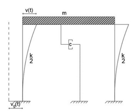
Figure 1. Newmark-β illustration
\[m\ddot{v} + c\dot{v} + kv = P_{eff} \tag{1}\]
\[m\ddot{v} + c\dot{v} + kv = -m\ddot{v}_a \tag{2}\]
; \(\ddot{v}\) is the acceleration, \(\dot{v}\) is the velocity, v is the displacement, and \(\ddot{v}_q\) is the ground acceleration.
Seismic response coefficient (\(C_S\)) is needed to calculate the design base shear based on static equivalent analysis. The formula is using the fundamental period, as follows.
\[C_{S-natural} = \frac{S_{D1}}{T\left(\frac{R}{I_0}\right)} \tag{3}\]
Based on SNI 1726:2019 (SNI 1726, 2019), the value of \(C_{S-natural}\) should not be less than,
\[C_{s\text{-minimum}} = 0.044 \ S_{DS}I_e \ge 0.01\] (4)
\(S_{DS}\) = acceleration parameter of short-period design spectrum response
\(S_{DS1}\) = acceleration parameters of 1-sec period design spectrum response
S<sub>1</sub> = acceleration parameters of the mapped design spectrum response
I<sub>e</sub> = primacy factor of earthquake
R = response modification factors
T = fundamental period of structure (seconds)
For performance analysis, the structural elements should refer to this ATC-40 capacity curve and based on TBI (TBI, 2017) and FEMA (FEMA 440, 2005) (FEMA P1050-2, 2015) (ASCE, 2017), the performance level of structure based on ground motion level is as follows Figure 1.
For structure reliability analysis, the probability of collapse can be determined by using lognormal
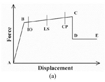
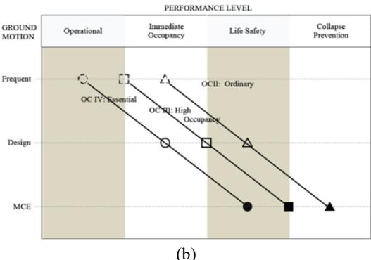
Figure 2. (a) Capacity curve ATC-40, (b) Performance Level
distribution. Parameters used in calculations are as
\[\zeta = \sqrt{\ln 2(1 + \Omega_f^2)} \tag{5}\]
; \(\zeta\) is standard deviation lognormal distribution
\[\Omega_{\rm f} = \sqrt{\Omega^2 + 0.15^2 + 0.15^2 + \left(\frac{\Omega}{\sqrt{n}}\right)^2} \tag{6}\]
\[\Omega = \frac{\sigma}{\mu} \tag{7}\]
; n is amount of data, \(\mu\) is mean values normal distribution, \(\sigma\) is standard deviation normal distribution.
\[\lambda = \ln \mu - \frac{1}{2}\zeta^2 \tag{8}\]
To ensure that the data obtained were lognormally distributed, a Kolmogorov-Smirnov validity test was performed with a significant level, α, with a target of 0.05. The Kolmogorov-Smirnov test is considered eligible if it meets the following equation.
\[D_n < D_n^a \tag{9}\]
The maximum value of \(D_n\) can be obtained from,
\[D_n = \max[F_n(x_i) - S_n(x_i)]\] (10)
The \(D_n^a\) value is obtained by interpolation of the Kolmogorov- Smirnov table test.
Table 1. Kolmogorov-Smirnov Table Test
| • | ||||
|---|---|---|---|---|
| n\α | 0,20 | 0,10 | 0,05 | 0,01 |
| 5 | 0,45 | 0,51 | 0,56 | 0,67 |
| 10 | 0,32 | 0,37 | 0,41 | 0,49 |
| 15 | 0,27 | 0,30 | 0,34 | 0,40 |
| 20 | 0,23 | 0,26 | 0,29 | 0,36 |
| 25 | 0,21 | 0,24 | 0,27 | 0,32 |
| 30 | 0,19 | 0,22 | 0,24 | 0,29 |
| 35 | 0,18 | 0,20 | 0,23 | 0,27 |
| 40 | 0,17 | 0,19 | 0,21 | 0,25 |
| 45 | 0,16 | 0,18 | 0,20 | 0,24 |
| 50 | 0,15 | 0,17 | 0,19 | 0,23 |
| - > 50 | 1,07 | 1,22 | 1,36 | 1,63 |
| n > 50 | \(\sqrt{n}\) | \(\sqrt{n}\) | \(\sqrt{n}\) | \(\sqrt{n}\) |
Then, fragility curve for lognormal distribution function is as follows.
\[f_{cap}(x_i) = \frac{1}{\xi x_i \sqrt{2\pi}} \exp\left[-\frac{1}{2} \left(\frac{\ln x_i - \lambda}{\xi}\right)^2\right]\](11)
3. Methodology
The analysis method used to evaluate the performance of the structure consists of non-linear time history analysis (CSI ETABS, 2017) (CSI Perform 3D, 2016) and structure reliability analysis by using Mathcad. Before that, structural planning needs to be done according to the applicable design criteria and loading. (Budiono, 2017) (Imran, I., Hendrik, F., 2014) (SNI 1727, 2020) (SNI 2847, 2019). This research methodology adapts the requirements set out in the code mentioned in the literature study.
4. Analysis Results
The structure being analyzed is a 240-meter tall building consisting of 60 levels. The structural system is a
Figure 3. Methodology flow chart

Figure 4 Typical floor plan
reinforced concrete special moment frame with a typical layout, as depicted in the following picture (Figure 4).
The modified seismic response coefficient \((C_{S-M})\) is employed when the structure model is subjected to the Risk-Targeted Maximum Considered Earthquake (MCE<sub>R</sub>). It is calculated as the average of the C<sub>S-natural</sub> and the C<sub>S-minimum</sub>. Furthermore, the average seismic response coefficient values are varied in the range of multiplier factors from 0.8 to 1.2. All of the values should be bigger than 1.2 C<sub>S-natural</sub> (20% safety factor), to ensure that the analysis does not overly minimize the earthquake parameters. As a note, this calculation only applies to high-rise buildings with a natural period exceeding 6 seconds.
\[C_{S-M} = k \left\{ \frac{C_{S-minimum} + C_{S-natural}}{2} \right\}\] (12)
\[C_{S-M} \ge 1.2C_{S-natural} \tag{13}\]
Structural design preliminary produces the fundamental period and seismic response coefficient calculations as shown in this following Table 2 and Table 3.
Table 2. Calculation of fundamental periods and seismic response coefficients
| Tx | 7.038 | s | Ty | 6.873 | s |
|---|---|---|---|---|---|
| Ta min | 2.9756 | s | Ta min | 2.9756 | s |
| Ta max | 4.1659 | s | Ta max | 4.1659 | s |
| Cs max | 0.0868 | Cs max | 0.0868 | ||
| Cs natural | 0.0113 | >0.01 | Cs natural | 0.0116 | >0.01 |
| Cs min | 0.0267 | Cs min | 0.0267 | ||
| 1.2Cs natural | 0.0136 | 1.2Cs natural | 0.0139 | ||
| CS-M (k=0.8) | 0.0190 | >1.2Cs natural | CS-M (k=0.8) | 0.0192 | >1.2Cs natural |
| CS-M (k=0.9) | 0.0152 | >1.2Cs natural | CS-M (k=0.9) | 0.0153 | >1.2Cs natural |
| CS-M (k=1) | 0.0171 | >1.2Cs natural | CS-M (k=1) | 0.0172 | >1.2Cs natural |
| CS-M (k=1.1) | 0.0209 | >1.2Cs natural | CS-M (k=1.1) | 0.0211 | >1.2Cs natural |
| CS-M (k=1.2) | 0.0228 | >1.2Cs natural | CS-M (k=1.2) | 0.0230 | >1.2Cs natural |
Table 3. Information of cs curve vs T
| Symbol | Cs Value | T (s) | |
|---|---|---|---|
| Cs min | 0.026729 | 1.15 | |
| Cs max | 0.086783 | 0.45 | |
| Cs natural | 0.011315 | 7.038 | |
| CS-M (k=0.8) | 0.022827 | 1.65 | |
| CS-M (k=0.9) | 0.020924 | 1.88 | |
| CS-M (k=1) | 0.019022 | 2.02 | |
| CS-M (k=1.1) | 0.017120 | 2.15 | |
| CS-M (k=1.2) | 0.015218 | 2.51 |
| Symbol | Cs Value | T (s) | |
|---|---|---|---|
| Cs min | 0.026729 | 1.15 | |
| Cs max | 0.086783 | 0.45 | |
| Cs natural | 0.011315 | 6.873 | |
| CS-M (k=0.8) | 0.022990 | 1.55 | |
| CS-M (k=0.9) | 0.021074 | 1.78 | |
| CS-M (k=1) | 0.019158 | 1.92 | |
| CS-M (k=1.1) | 0.017242 | 2.05 | |
| CS-M (k=1.2) | 0.015326 | 2.41 |
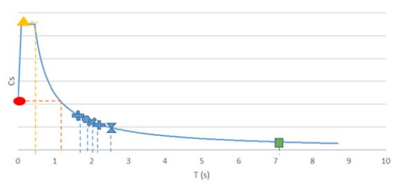
Figure 5. Illustration of seismic response coefficient
The Figure 5 shows that the value of the modified seismic response coefficient (CS-M) is between the CSnatural and the CS-minimum.
5. Non-Linear Time History Analysis Result
The results consist of inter-story drift, residual drift, and plastic joint damage. Inter-story drift is a relative
TBI arthquake level Lateral Drift Limit SNI TBI MCER 2% 3% SLE - 0.5%
Table 4. Inter-story drift requirements based on SNI and displacement between floors where the zero-point reference is below the observed floor. (TBI, 2017)
Based on TBI section 6.7.3, for each floor, the absolute average value of the residual drift must not exceed 0.01. Residual drift is inter-story drift which occur at the end of the earthquake phase. These limits are intended to prevent excessive deformation in the aftermath of an earthquake which will cause a great danger to the surrounding construction in the event of a strong aftershock.
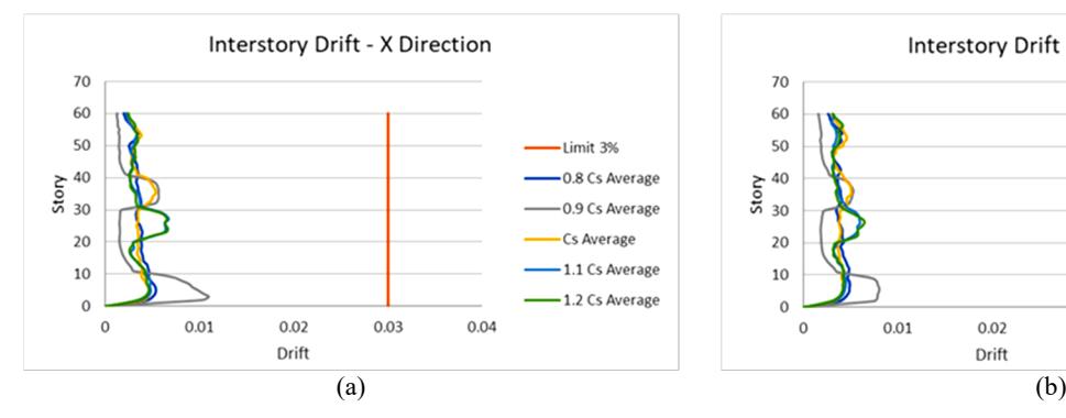
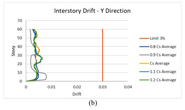
Figure 6. Inter-story Drift: (a) X Direction, (b) Y Direction
Figure 7. Residual drift: (a) X direction, (b) Y direction
Table 5. Results of plastic joint damage checking
| Case | Performance Level | |||||||
|---|---|---|---|---|---|---|---|---|
| No | Dir. | SLE | CS-M (k=0.8) | CS-M (k=0.9) | CS-M (k=1) | CS-M (k=1.1) | CS-M (k=1.2) | |
| X | 0.09147 IO | 0.529 CP | 0.505 CP | 0.9752 LS | 0.8615 LS | 0.5205 LS | ||
| 1 | "Kern County" | Y | 0.8779 Yield | 0.542 CP | 0.508 CP | 0.9885 LS | 0.796 LS | 0.413 LS |
| X | 0.6128 Yield | 0.6487 CP | 0.6277 CP | 0.5208 CP | 0.9981 LS | 0.7184 LS | ||
| 2 | "El Alamo" | Y | 0.6607 Yield | 0.6062 CP | 0.5908 CP | 0.57 CP | 0.5578 CP | 0.8544 LS |
| X | 0.3766 Yield | 0.7804 CP | 0.7696 CP | 0.756 CP | 0.655 CP | 0.5999 CP | ||
| 3 | "Tabas_Iran" | Y | 0.5179 Yield | 0.9334 CP | 0.8185 CP | 0.7403 CP | 0.732 CP | 0.7266 CP |
| X | 0.2997 IO | 0.655 CP | 0.6245 CP | 0.5829 CP | 0.5471 CP | 0.5271 CP | ||
| 4 | "Loma Prieta" | Y | 0.3488 IO | 0.6642 CP | 0.6331 CP | 0.5702 CP | 0.5437 CP | 0.9334 LS |
| X | 0.4822 IO | 0.9261 CP | 0.8479 CP | 0.783 CP | 0.7576 CP | 0.5554 CP | ||
| 5 | "Kobe_ Japan" | Y | 0.3933 IO | 0.8846 CP | 0.8264 CP | 0.7597 CP | 0.7298 CP | 0.5554 CP |
| X | 0.5033 Yield | 0.7163 CP | 0.5806 CP | 0.5576 CP | 0.8929 LS | 0.8536 LS | ||
| 6 | "Hector Mine" | Y | 0.303 Yield | 0.6766 CP | 0.6638 CP | 0.6368 CP | 0.546 CP | 0.9672 LS |
| X | 0.4317 Yield | 0.8623 CP | 0.7321 CP | 0.6534 CP | 0.6253 CP | 0.4769CP | ||
| 7 | "Duzce_Turkey" | Y | 0.01025 Yield | 0.8716 CP | 0.6705 CP | 0.5911 CP | 0.5813 CP | 0.4594 CP |
| "Chuetsu-oki_ | X | 0.5528 IO | 1.05 CP | 0.9259 CP | 0.8165 CP | 0.7781 CP | 0.7525 CP | |
| 8 | Japan" | Y | 0.6162 IO | 1.107 CP | 1.058 CP | 0.8371 CP | 0.8086 CP | 0.5645 CP |
| X | 0.1508 IO | 0.5505 CP | 0.5283 CP | 0.5273 CP | 0.8527 LS | 0.7135 LS | ||
| 9 | "Iwate_ Japan" | Y | 0.1518 IO | 0.5295 CP | 0.9964 LS | 0.9769 LS | 0.7958 LS | 0.6258 LS |
| "El Mayor | X | 0.0069 Yield | 0.5814 CP | 0.5254 CP | 0.9623 LS | 0.858 LS | 0.804 LS | |
| 10 | Cucapah_ Mexico" | Y | 0.7643 Yield | 0.5389 CP | 0.5347 CP | 0.5197 CP | 0.5139 CP | 0.9722 LS |
| "Darfield_ New | X | 0.0008 Yield | 0.7329 CP | 0.5688 CP | 0.5343 CP | 0.5341 CP | 0.9999 LS | |
| 11 | Zealand" | Y | 0.0097 Yield | 0.6879 CP | 0.6014 CP | 0.5762 CP | 0.5616 CP | 0.9735 LS |
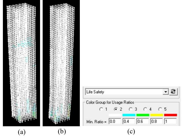
Figure 8. Final condition of 1.2 cs average model – el alamo: (a) X dir, (b) Y dir, (c) colour group
The figures above show that inter-story drift and residual drift do not exceed the required limits. Then, results summary of checking the damage to plastic joints in the final condition of each model after the earthquake force is given in the following table.
Hence, results summary of checking the damage meet the required performance level based on Figure 2b. The greatest damage of the structural elements when earthquakes applied is dominated by beams, then shear walls and columns.
6. Structure Reliability Analysis Result
For this analysis, PGA (earthquake acceleration) for each case will be scaling up incrementally until the structure is collapse. Then, the probability of collapse can be determined by using lognormal distribution as mentioned in study of literature. Based on the
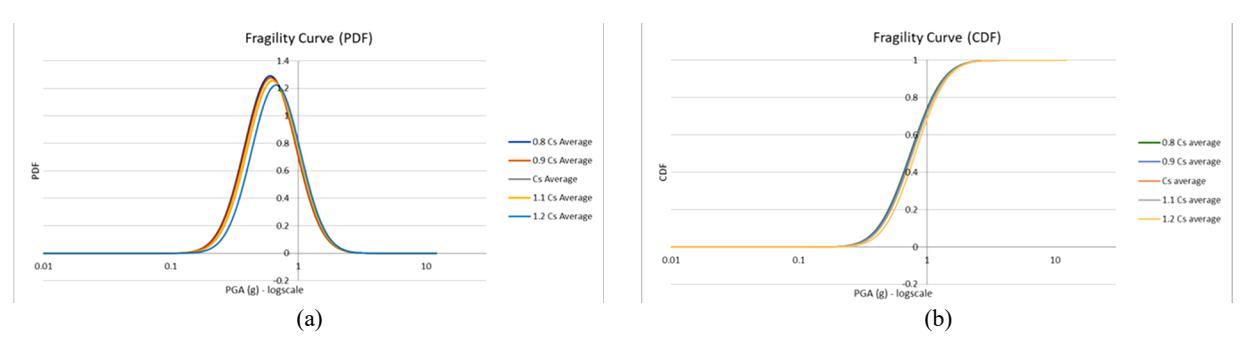
Figure 9. Fragility curve: (a) (PDF), (b) (CDF)
Table 6. Probability of collapse (11 PGA data)
| Return Period - | Cs modified | ||||
|---|---|---|---|---|---|
| Return Period — | 0.8 Cs ave | 0.9 Cs ave | Cs ave | 1.1 Cs ave | 1.2 Cs ave |
| Annually | 1.243 X 10⁻⁴ | 1.198 X 10⁻⁴ | 1.082 X 10⁻⁴ | 9.044 X 10⁻⁵ | 7.957 X 10⁻⁵ |
| 50 Years | 6.195 X 10⁻³ | 5.973 X 10⁻³ | 5.393 X 10⁻³ | 4.512 X 10⁻³ | 3.971 X 10⁻³ |
calculation, the lognormal distribution function fulfills the requirements of \(D_n < D_n^a\). The fragility curve for each structural model based on the lognormal distribution as shown the Figure 9.
Then the risk of structure failure calculated by using risk integral method. The polynomial equation fitting with seismic hazard curve used is a level 6 equation as follows. (J. A. Patrisia et al., 2017)
\[\ln NPGA = -4.2331 \times 10^{-5} (\ln PGA)^6 - 0.00189 (\ln PGA)^5 - 0.0329 (\ln PGA)^4 - 0.301 (\ln PGA)^3 - 1.738 (\ln PGA)^2 - 6.832 (\ln PGA) - 13.3\] (17)
\[NPGA = P(PGA > x) \tag{18}\]
\[P(collapse) = \int_{0}^{\infty} P(PGA > x) \frac{dP[f_{cap}(PGA = x)]}{dx} dx\] (19)
\[P(collapse in Y years) = 1 - [1-P(collapse)]^{Y}\] (20)
: Y = 50
Integration calculations are performed numerically using the Math-Cad application for each structural model, as follows.
\[f(x) = \frac{1}{\xi x \sqrt{2\pi}} \exp\left[-\frac{1}{2} \left(\frac{\ln x_i - \lambda}{\xi}\right)^2\right]\] (21)
\[g(x) = P(PGA > x) = NPGA\] \[= \exp[-4.2331]\] \[\times 10^{-5} (\ln PGA)^{6}\] \[- 0.00189 (\ln PGA)^{5} - 0.0329 (\ln PGA)^{4}\] \[- 0.301 (\ln PGA)^{3} - 1.738 (\ln PGA)^{2}\] (22)
\(-6.832(\ln PGA) - 13.375\)
\[P(collapse) = \int_{-\infty}^{\infty} f(x)g(x)dx \tag{23}\]
The probability of collapse in 50 years is below 1% so it is an acceptable risk.
7. Conclusions
In conclusion, the findings of this study can be summarized as follows:
- 1. Based on verification through non-linear time history analysis, in general, the performance of structures by applying frequent or Service-Level Earthquake (SLE) and Risk-Targeted Maximum Considered Earthquake (MCE<sub>R</sub>) ground motions, meeting the requirements criteria of TBI 2017.
- 2. These results indicate the potential utility of the modified seismic response coefficient (C<sub>S-M</sub>).
- 3. However, it is important to note that the modified seismic response coefficient is not intended as a replacement for current methods in designing super high-rise buildings.