
Abstrak
Dalam makalah ini, diusulkan metode perencanaan dan analisis resiko peluang kegagalan struktur gagal-aman dari rangka baja dan beton akibat beban gempa. Struktur rangka tersebut merupakan bagian dari bangunan fasilitas nuklir, dan modus keruntuhannya direncanakan mengikuti mekanisme kegagalan balok secara aman. Mekanisme gagal-aman dicapai dengan mengarahkan terbentuknya sebagian besar sendi plastis di balok dan hanya beberapa di kolom. Hanya jenis kegagalan lentur yang diijinkan terjadi pada balok dan harus dihindari jenis kegagalan selainnya semisal gagal geser, takuk lokal atau tekuk torsi lateral. Pada makalah ini dipelajari dua jenis struktur rangka gagal-aman yaitu struktur rangka pemikul momen khusus (SRPMK) dan struktur rangka pemikul momen biasa (SRPMB). Tatacara perencanaan dijelaskan secara rinci, dan peluang kegagalan berdasarkan kerentanan dihitung dan dibandingkan diantara kedua jenis struktur tersebut. Analisis riwayat waktu taklinier dilakukan untuk mengkaji kinerja stuktural keduanya. Hasil perhitungan menunjukkan bahwa SRPMB gagal-aman menghasilkan peluang kegagalan yang lebih rendah daripada SRPMK gagal-aman. SRPMB rangka baja menunjukkan kinerja yang sangat memuaskan.
Kata-kata Kunci: Gagal-aman, struktur rangka beton dan baja, kerentanan, peluang kegagalan, kegempaan, analisis riwayat waktu.
1. Introduction
The seismic design of structures, systems, and components (SSC) of nuclear facilities are regulated by ASCE/SEI 4-16 (ASCE, 2017), ASCE/SEI 43-2019 (ASCE, 2019), and IAEA/SSG-67-2021 (IAEA, 2021) provisions. In the provisions, the use of standard building codes such as ASCE/SEI 7-22 (ASCE, 2022) are allowed for certain structures belonging to Seismic Design Category 4 with the probability of failures in the order of less than 10-3 per annum (IAEA, 2021). For higher seismic design categories with lower probability of failures, there are no special codes to follow, except that the probability of failures shall be demonstrated to be less than the respective performance goal. In this study, the concept would be applied to seismic resistant frame structures designed to serve in the environment of nuclear power plants (NPPs) based on the standard code requirements and improved them such that the failure probabilities meet that required by the NPP standards. Not only does the failure probability meet the NPP standards, but also, if it ever collapses due to seismic events it would do so in the safe-to-fail modes.
Based on conventional seismic codes, e.g., ASCE/SEI 7-22, it is possible to design moment-resisting frame
structures for three categories, i.e., Ordinary Moment Frame (OMF), Intermediate (IMF), and Special (SMF). The last one poses the most stringent requirements such as 1) plastic hinges should develop mainly or merely at beams ends; 2) steel sections shall be seismically compact with short braced length in terms of lateral-torsional buckling, or well detailed/ confined for concrete; 3) all kinds of premature failures such as lack of shear capacity shall be avoided. But the OMF does not share the requirements and therefore is unsuitable for seismic resistant structures in sites with moderate to high seismic risks. There are ways, however, to improve the code OMF so that it can withstand seismic forces safely, with less stringent requirements than those of the SMF. The improved OMF is referred to as the safe-to-fail OMF; and the terminology applies to the SMF as well, when appropriate. The objective of the paper is therefore to establish the safe-to-fail model (SM). The safe-to-fail model is basically developed based on the code model which is then improved sufficiently to satisfy those three requirements. For instance, the steel safe-to-fail OMF shares the section compactness of the code OMF which is less stringent than that of the code SMF; similarly, the RC safe-to-fail OMF beam sections are detailed and reinforced for shear in less restrictive manner than the RC code SMF. In this way, it can be ensured that the safe-to-fail OMF remains less heavily detailed than that of the code SMF while maintaining its seismic performance required by NPPs standards.
The safe-to-fail idea has been around for a while. Ahern (2011) suggested the adoption of safe-to-fail design philosophy, instead of the fail-safe design concept. This means designing structures to be safe in case of structural failures, rather than aiming to prevent them altogether, which is consistent with the current seismic design philosophy adopted in standard building codes (ASCE, 2022). This safe-to-fail concept is also supported by Kim et. al. (2019), particularly in designing structures to withstand natural hazards such as earthquakes. Historically a kind of safe-to-fail concept was coined around the 1970s in New Zealand in the form of capacity design for reinforced concrete frames (Park and Paulay, 1975). In capacity design, plastic hinges were intended to form in beams ends, and those in columns were to be avoided (it was expected that beam plastic hinges would dissipate seismic energy more stable than those of the columns'). This was achieved by requiring a ratio of the plastic moment sum of the column sections (considering the axial loads) to those of the adjoining beams or shortly strong column-weak beam (SCWB) ratio to be 2-3. All other but flexural failure shall be avoided by supplying sufficiently high shear capacity and well detailed/confined sections. In the United States, similar approach was introduced in SEAOC (1973) and ACI (1971). The approach was referred to as the strong column-weak beam design with the SCWB ratio of around 1.2. However, presently there are no codes that adopt the capacity design with SCWB ratio of 2-3. The ACI 318-19 (2019) specifies 1.2, the Eurocode 8 (CEN, 2004) 1.3, and the New Zealand NZS 3101 (NZS, 2006) code requires more than 1.3 but not higher than 1.8. It was desired that beams sections fail in flexural modes prior to failure of the adjoining column sections while no other premature failure modes were allowed. For the discussions herein, the authors proposed to refer the code's requirement of the SCWB ratio 1-2 as the strong column-weak beam design, the capacity design with SCWB ratio 2-3, and the safe-to-fail design with SCWB ratio of 3-4. In this context, the safe-to-fail design will produce the most robust frames, when no premature failures but the flexural exist. This is achieved by proper design/detailing and strengthening, if needed, so that premature failure modes can be avoided.
Concerns regarding the occurrence of plastic hinges in columns despite having a relatively high SCWB ratio have already been reported in earlier studies (Priestley and Calvi, 1992; Bondy, 1996; Lee, 1996). The research supports the SCWB ratio to be two for uniaxial bending and three for biaxial (ACI, 2002). Haselton et al. (2011) suggested the ratio should be higher than three, or even four (Kuntz and Browning, 2003; Moehle, 2014). Mangkoesoebroto et al. (2019) found 3.5, while Rianto (2020) discovered 2.9 for steel safe-to-fail frames. Despite this fact, the codes maintain lower values due to economic arguments (e.g., ACI, 2002), and they do not ensure that columns will not yield or suffer damage when frames must sustain inelastic seismic loads, and therefore need to be detailed (Moehle et al., 2008). In contrast, the safe-tofail design must ensure that there will not be columns plastic hinges, except a few at their bases, and therefore the column detailing is not of primary concerns. The collapse mode of the safe-to-fail design is therefore expected to be a beam-sidesway mechanism with few column plastic hinges formation especially at their bottoms and tops. The consequence of this type of collapse mechanism is that the interstory drift ratios are rather uniformly distributed along the stories and about the same as the total story drift. Therefore, the inter-story drift ratio might not be a suitable damage measure in this case. In this study, the ratio of the number of the developed beam plastic hinges with respect to the number of the potential beam plastic hinges was used as the damage measure. A fifty percent ratio was used associated with the median value of collapse probability.
The structures were excited by a suite of ground accelerations with three components. All ground accelerations were spectrally matched to a site-specific smooth spectrum. Following the incremental dynamic analyses (IDA) for structures with the fundamental periods of \(T_1\), the capacity curves relating the base shear coefficients to the spectral acceleration at \(T_1\) (S<sub>a</sub> \((T_1)\)) can be constructed (Vamvatsikos and Cornell, 2002). Capacity curves were essential for assessing the performance or the collapse mechanism of structures. Based on this curve, another curves, the fragility curves, expressing the conditional probability of collapse of the structures at any given \(S_a(T_1)\) could be derived. Because the spectral accelerations have their own probability of occurrence defined by their hazards, the probability of collapse can only be determined by the convolution of the fragility and the hazard curves.
The collapse probability will be used as a sole metric in evaluating the performance of the structures.
In this study, four types of framed structures with the same skeleton were evaluated and compared based on their probabilities of collapse. The structures were of steel and concrete; ones were of the ordinary moment open frames and the others were special ones all with fixed bases. All of them were of safe-to-fail type, i.e., their SCWB ratios were 3-4. The structures were parts of the nuclear facility located in Bandung, Indonesia. The objective was to decide which structure was the most appropriate to be constructed in the nuclear environment.
The organization of the study was preceded by evaluating the seismicity and ground motions at the site. The site was situated in the vicinity of the Lembang active fault, and therefore its associated hazard needed to be defined. The discussion would then be followed with the beam sectional designs focusing on the momentcurvature relations and the ductility capacity prior to their collapse states at that section. While the collapse state of beams was dictated by their ductility ratio, the collapse of the structures was determined by the number of the collapsed beams. Therefore, the collapse criterion of the structure was defined based on the latter. Next, the model or the skeleton of the structures and its design will be discussed in detail. Four variants of ordinary and special moment frames, as well as the steel and concrete materials will be covered both for ones based on codes and, the other, based on their strengthened models to satisfy the safe-to-fail criterion. The structural fragility and the probability of collapse are discussed afterward prior to the concluding remark.
2. Site Seismicity and Ground Motions
Seismic study of the site has been performed to produce hazard and spectral curves (Mangkoesoebroto et al., 2019). They were obtained by considering both the probabilistic and deterministic aspects of the seismotectonic scenario based on the surrounding site. The peak ground acceleration (PGA) for the maximum credible earthquake (MCE) was 0.35g (H) and 0.26g (V) for mean plus sigma confidence level. Their square root of the sum of the squares (SRSS) combination became 0.44g (mean plus standard deviation), and was used as the basis in the design processes. The corresponding median values for the MCE was 0.24g (H), 0.17g (V) and the SRSS combination of
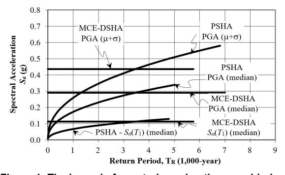
Figure 1. The hazard of spectral acceleration considering probabilistic and deterministic scenarios for median and mean plus sigma values. \(T_1\)=1.3s; PGA=\(S_a(T=0)\)
0.29g (median). The median values were used as the basis for seismic evaluation processes. The spectral acceleration at the fundamental period of \(T_1\) can also be determined for the maximum deterministic, i.e., 0.11g (median) (\(T_1 = 1.3\)s was determined based on the first mode in this study). All curves are plotted in Figure 1 together with the results of the probabilistic analyses. It is observable that the MCEs are associated with a 3.500-year return period. By defining that hazard \(H(a)=1/T_R\), where \(T_R\) is the return period, the hazard is replotted in Figure 2 for median level. The hazard in this form will be convoluted with the fragilities to determine the probability of failures.
The response spectra were developed by the same notion. They are shown in Figure 3 for the SRSS combinations of the horizontal and vertical components for median and mean plus sigma levels. The latter were employed in the response spectrum structural designs while the former for the risk analyses. This is in accordance with IAEA (2021). The peak ground accelerations are the same as the MCEs for the respective levels.
As required (ASCE, 2022), eleven earthquake records with spectral shape close to that of the target (the median value in Figure 3) were downloaded from PEER (2022) and listed in Table 1. The records were spectrally matched at frequency range of 0.1-25 Hz (0.4 \(\leq T\) (s) \(\leq 10\)), which satisfied the requirements of ASCE/SEI 7-22, with the resulting spectra shown in
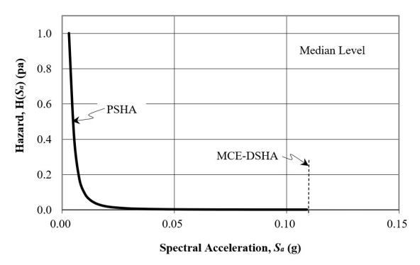
Figure 2. Median hazard for spectral acceleration at \(T_1\)=1.3s (MCE<sub>M</sub> = 0.11 g).
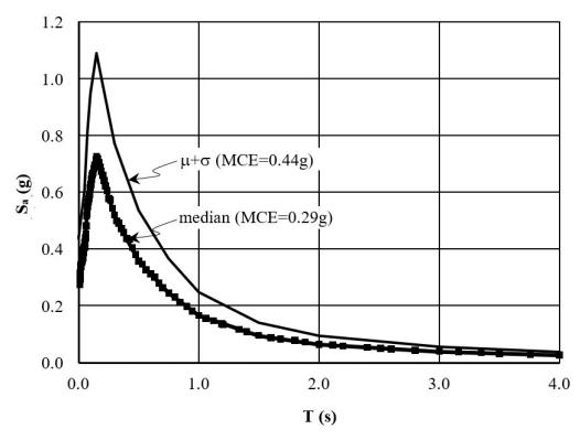
Figure 3. The spectral acceleration considering the probabilistic and deterministic scenarios (SRSS combination for horizontal and vertical directions). Matched earthquake records spectrum almost coincides with the median level
Figure 3. Though their spectra almost coincide with the (median) target spectrum, they still differ in their phase angles and the ratios among their threecomponent. The matching procedure was performed in three dimensions, and the phase angles as well as the component ratios of the recorded records were maintained (Mangkoesoebroto et al., 2023).
3. Sectional Moment-Curvature and Collapse Criterion
In this study, the allowable structural failure is governed by the formation of plastic hinges in beams alone, and a few at the column bases; any other mode of failure (e.g., shear, buckling, torsion) must be avoided. It is therefore essential to discuss the beam section moment-curvature relations as it determines the property of the plastic hinge. Two types are considered: one for the ordinary moment frame (OMF) structures, and the other for the special moment frames (SMF). They differ in terms of capacity and ductility. For steel frame structures, the maximum ductility at collapse prevention (CP) is adopted as 2.2 for OMF and 5 for SMF. Assuming that damage is affected more by the ductility ratio rather than the initial stiffness, then their damage state at collapse is different, being more severe for the SMF at ductility of 5 than that of OMF at ductility of 2.2. Figure 4 presents such relations for typical two beam sections used in the study. On the left the OMF beam section shows higher capacity but lower ductility; the otherwise is true for the SMF section. However, both sections show the same relations in the dimensionless units (right). And they are modeled to have significantly reduced capacity when their maximum ductility is achieved. Based on these momentcurvature relations, nonlinear behavior of the structures is modeled using concentrated hinges at the ends of beam and column members, with consideration of axial load for columns, while the members are modeled as elastic line elements.
The damage measure (DM) is the collapse indicator of the structures. The commonly used DM was the interstory drift angle, however, because in safe-to-fail structures the inter-story drift angles may not vary appreciably, in this study a different definition of collapse is employed. The structures were defined at collapse state when they developed fifty percent (median level) of plastic hinges of the total potential hinges; the remaining plastic hinges might be of lower ductility than the first fifty percent. This DM definition is consistent with the collapse mechanism of a safe-tofail frame defined herein. Figure 5 shows the typical collapse of both SMFs and OMFs, albeit they might show different configurations. Thus, at collapse, the SMF structures will show as many plastic hinges as that of the OMFs, however, the (curvature) ductility and therefore the damage severity is different, being more severe for SMFs. It is therefore expected that the OMF structures are more robust than the SMFs. In the analyses the inter-story drift angles were computed and compared, as well.
When the structure attained the collapse configuration shown in Figure 5, it was assigned a high probability of failure of 95% or over, or mathematically
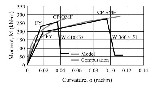
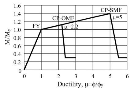
Figure 4. Typical moment-curvature relation for two steel sections. On the left, one for OMF section is of WF 410x53 with maximum ductility of mmax=2.2; and the other for SMF is for WF 360x51 with mmax=5. On the right, shown in the dimensionless units, they coincide into one relation. (FY= first yield; CP=collapse prevention; WF=wide flange; OMF=ordinary moment frame; SMF=special moment frame; m=ductility ratio.)
Table 1. Earthquake data and their properties*)
| Event | Origin | Date | Station | PGA (g) | Mw | Rjb (km) |
|---|---|---|---|---|---|---|
| El Mayor-Cucapah | Mexico | 2010 | Michoacan | 0.83 | 7.2 | 13 |
| Erzican | Turkey | 1992 | Erzinican | 0.50 | 6.7 | 10 |
| Imperial Valley-07 | USA | 1979 | El Centro 6 | 0.29 | 6.5 | 7 |
| Imperial Valley-06 | USA | 1979 | Calexico | 0.29 | 6.5 | 7 |
| Kobe | Japan | 1995 | Takatori | 0.81 | 6.9 | 15 |
| Mammoth Lakes-02 | USA | 1980 | Mammoth Lakes | 0.51 | 6.0 | 7 |
| N. Palm Springs | USA | 1986 | DHSP 517 | 0.74 | 6.0 | 10 |
| Parkfield | USA | 1966 | Temblor | 0.38 | 6.2 | 9 |
| Chi-Chi | Taiwan | 1999 | CHY010 | 0.25 | 7.6 | 20 |
| Darfield | New Zealand | 2010 | SPFS | 0.22 | 7.0 | 30 |
| Iwate | Japan | 2008 | Semine Kurihara City | 0.19 | 6.9 | 29 |
*) The records were selected based on their spectral response closeness to the target; Mw: moment magnitude; PGA: peak ground acceleration; Rjb: Joyner-Boore distance
122 Jurnal Teknik Sipil
\(P[S_a \le S_{a.95,CP}^{50}] \ge 0.95\), where \(S_{a.95,CP}^{50}\) is the spectral acceleration to cause the formation of plastic hinges as much as 50% of the total potential plastic hinges, or median level; they are of being CP (collapse prevention), and the collapse probability is assumed to be 95% or over. This is applicable for both OMFs and SMFs structures. In general, the spectral acceleration is expressed as \(S_{a,95,[.]}^{50}\) where the index [.] is substituted for
CP or FY as appropriate for the collapse prevention or the first yield, respectively. The latter means that there is high probability of occurrence of the first yield point.
4. The Model of the Structures and Its Design
Regular open frame structures were studied in the study. Though the skeletons are identical, the structures are once made up of steel and the other of RC. The steel structures have four variants, i.e., two for OMFs both designed strictly based on codes and then they were strengthened to comply with the safe-to-fail criterion; and, similarly for SMFs. The RC structures were also treated the same way. Thus, in total, there were eight variants designed and investigated, of which four of them (all of safe-to-fail models) were, later, subjected to eleven three-dimensional ground motions, completing forty-four incremental nonlinear time history analysis computer runs.
Figure 6 presents the model structure worked out herein. It consists of eight-story (28.5 meters height), four-bay in x-direction (@ 6 meters), and six-span in y-axis (@ 5 meters), the bases are all fixed, and all connections are rigid joints. The structure sustains live load, self-weight and superimposed dead, as well as seismic loads. In accordance with ASCE/SEI (2022), the live load is 2.5 kN/m<sup>2</sup> for typical floors and 1 kN/m<sup>2</sup> for roof, while the superimposed dead is 0.9 kN/m<sup>2</sup> for typical floors and 0.6 kN/m<sup>2</sup> for roof, respectively.
The design of RC code models was performed strictly based on ASCE (2022) for gravity and seismic loads procedures (ACI, 2019, for concrete; and AISC, 2016a & 2016b, for steel frames). The response spectrum design was performed based on the mean plus sigma response spectra shown in Figure 3. The code maximum demand as well as the minimum requirements dictated the capacities of the structures were all satisfied.
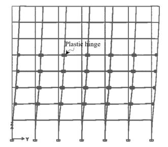
Figure 5. The state of collapse of typical structures is defined as the formation of fifty percent (median level) plastic hinges of the total potential hinges. The hinge is of \(\mu_{\text{max}}\text{=}2.2\) and 5 for OMFs and SMFs, respectively. The other beams ends might be populated by plastic hinges but of lower ductility than those of collapse preventions (not shown)
The steel structure was designed in accordance with AISC (2016a & 2016b). The resulting sections for steel material of ASTM A36 are shown in Table 2 for both OMF and SMF, referred to as the code model (CM), herein. Subsequently, the structures were excited by the spectrally matched (median level) ground motions based on the earthquake records listed in Table 1. In time history analyses only 30% of live load was registered, while the other loads were the same. To satisfy the failure criterion set forth in Section 3 for an up scaled PGA level to reach the failure or CP point, a strengthening as well as detailing steps needed to be carried out. The corresponding results for the strengthened sections are shown in the same Table 2, referred to as the safe-to-fail model (SM).
The response modification factor for OMF is lower than for SMF, causing the former to sustain higher seismic base shear. Consequently, the section sizes used for OMF tend to be heavier or, at least, the same as that for SMF. Notice in Table 2 that the beam sections for OMF are stronger than that for SMF, both for the code and the safe-to-fail models. As for the columns, the section slenderness requirements of the code for SMF have caused those thick-walled square cross sections to be used for the columns; however, the requirements for OMF are not as stringent, although both are compact sections. This fact is observed in the table as thinner column sections are employed for the OMF. The case is the same for both the code and safe-to-fail models. The columns for the safe-to-fail model are the heaviest because no plastic hinges are allowed to form in columns. The SCWB ratio was 2.9 or up for the safe-tofail models both OMF and SMF, higher than that required by the code of 1.0 for SMF. Despite this fact, however, their weights are comparable being heaviest for the SMF due to, among other, the section slenderness ratio requirements. Consistent with these conditions, the fundamental period is lower for OMF than for SMF, and the lowest for the safe-to-fail model. This means that the OMF safe-to-fail model has the highest stiffness among them all.
The concrete structures were treated similarly and were designed according to the ACI (2019). Table 3 shows the results for OMF and SMF as well as CM and SM computations. It was possible to set them to have components of the same dimensions and differ only in the number of reinforcements. Therefore, they may have the same weight and the fundamental periods. The periods were computed based on the crack sections specified by the code. From the table it is observable that there is not much difference in the number of reinforcements for the girders between the code and the safe-to-fail models. However, the reinforcements are more for OMF than SMF due to higher base shear demand for the former (OMF has lower response modification factor than SMF). The reinforcements for columns are more for the safe-to-fail than for the code models to ensure that no plastic hinges were developed in columns unless at bases. The computed SCWB ratio was 3.6 or up for the safe-to-fail model both for OMFs and SMFs, consistent with other investigations of 3-4 (Haselton et al., 2011; Kuntz and Browning, 2003). The ratio was higher than the code requirement of 1.2 for
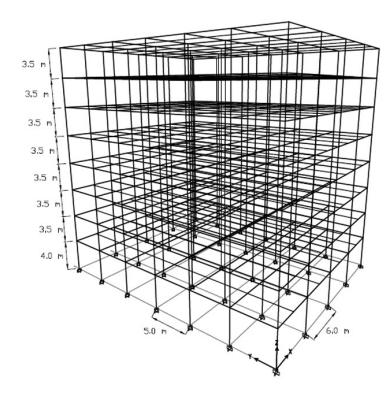
Figure 6. The model of the structure: 8-story (28.5 meters high), four-bay in x-direction (24 meters), and six-span in y-direction (30 meters). Bases are all fixed, and all connections are rigid joints
SMF. During the design process, the code minimum reinforcements were all satisfied.
5. Structural Fragility
The four variants of the safe-to-fail models, i.e., two for steel and concrete and two for OMFs and SMFs, could satisfy the failure criterion outlined in Section 3. The frames were subjected to eleven three-component earthquake acceleration input motions listed in Table 1. The spectral acceleration spectra of each earthquake matched that of the median spectrum shown in Figure 3 at all periods. The major direction of the motions was aligned with the weak axis of the structures. The peak ground accelerations (PGA) were up scaled incrementally until the frames achieved the plastic hinge configuration shown in Figure 5 defined as the state of collapse if the hinges were that of CP level, and the state of yielding if the hinges were that of FY (see Figure 4). The spectral acceleration at the structural fundamental period associated with CP was designated as \(S_{a.95,\text{CP}.i}^{50}\), and that associated with FY as \(S_{a.95,\text{FY}.i}^{50}\) due to the \(i^{\text{th}}\) earthquake record. The base shear and the top story lateral displacement were also registered. Repeat this computation for all earthquake records in the list and obtain their geometric mean as the median values for the spectral acceleration at CP and FY levels, namely \(S_{a.95.\mathrm{CP}}^{50}\) and \(S_{a.95.\mathrm{FY}}^{50}\), the base shear, as well as the displacement.
Thus, in this way it was possible to create the spectral acceleration dependent capacity curve with two points, i.e., FY and CP points. The curves relating the maximum base shear as ordinate versus the spectral acceleration and the maximum top story lateral displacement as abscissas were shown in Figure 7 (solid lines).
It was defined that the probability of collapse at CP was 95% or over, i.e., \(P[S_a \leq S_{a.95,\text{CP}}^{50}] \geq 0.95\). In this way, one point on the fragility curve was fixed. Another point in the curve was the design point. The point was associated with the level deemed safe enough to design the elastic capacity of the frame; and was defined as the FY level divided by a safety factor, SF. At the point, the probability of failure was assigned a low value of 5% or lower, or \(P[S_a \leq S_{a.05,\text{CP}}^{50}] \leq 0.05\).
Since FY point was related to CP by ductility \((\mu)\), then, \(S_{a.05,\text{CP}}^{50} = S_{a.95,\text{CP}}^{50}/R\), where \(R = \mu\) x SF is the response modification factor. The value of SF=1.6 for flexural failure (Mangkoesoebroto et. al., 2019) was used to define the ductility \((\mu)\) in this study given R was identified from the codes. Both the design and the CP points were employed to determine the two parameters involved in the lognormal fragility curves; thereby defining a unique relationship between the capacity and the fragility curves.
The fragility curve, assumed to be lognormal (Kennedy and Ravindra, 1984), is a conditional probability relationship between the probability of occurrence and the earthquake intensity measures (IM). The lognormality of the structural fragility relations was discussed, among others, by Erberik and Elnashai
Table 2. Steel component sections (ASTM A36) and other properties
| Components | Floors | OMF | SMF | ||
|---|---|---|---|---|---|
| 1-5th | □ 457.2x457.2x12.7 | □ 457.2x457.2x28.6 | CM | ||
| Columns | 1-3 | □ 558.8x558.8x19.1 | □ 457.2x457.2x28.6 | SM | |
| Columns | 6-8th | □ 355.6x355.6x11.1 | □ 355.6x355.6x22.2 | CM | |
| 0-8 | □ 457.2x457.2x15.9 | □ 355.6x355.6x28.6 | SM | ||
| W 460x60 | W 410x60 | CM | |||
| x-direction | (455x153x8x13.3) | (455x153x8x13.3) (406x178x7.8x12.8) | |||
| x-direction | W 460x60 | W 410x60 | SM | ||
| Girders | (455x153x8x13.3) | (406x178x7.8x12.8) | SIVI | ||
| W 410x53 | W 360x51 | CM | |||
| y-direction | (404x178x7.5x10.9) | (356x171x7.2x11.6) | |||
| y-direction | W 410x53 W 360x51 | SM | |||
| (404x178x7.5x10.9) | (356x171x7.2x11.6) | SIVI | |||
| Response modif | ication (R) | \(R=3.5, \mu=2.2\) | \(R=8, \mu=5\) | CM | |
| and ductility (µ) factors | \(R=3.5, \mu=2.2\) | \(R=8, \mu=5\) | SM | ||
| Fundamental pe | \(riod(T_1)\) | 1.41 s | 1.47 s | CM | |
| y-direction | 1.26 s | 1.45 s | SM | ||
| Total weight | 27.6 MN | 29.1 MN | CM | ||
| 28.8 MN | 29.4 MN | SM | |||
\(Units \ in \ mm; CM, SM: code \ and \ safe-to-fail \ models; \ OMF, SMF: \ ordinary \ and \ special \ moment \ frames; \ \Box, W: \ square \ hollow \ and \ wide-flange \ sections.\)
124 Jurnal Teknik Sipil
Table 3. RC component sections and other properties
| Components Strength | Story/floor Sizes | OMF | SMF | |
|---|---|---|---|---|
| Columns fc'=40 MPa | 1-5th | 28D16 (8D10-90) | 28D16 (8D10-90) | CM |
| 700/700 | 40D16 (8D10-90) | 40D16 (8D10-90) | SM | |
| 6-8th 600/600 | 20D16 (6D10-90) | 20D16 (6D10-90) | CM | |
| 32D16 (8D10-90) | 28D16 (8D10-90) | SM | ||
| 1-5' 350/7 x-direc 6-8' 350/6 Girders fc'=35 MPa y-direc 1-5' 300/6 y-direc 6-8' | x-direction | S:7D16/5D16 (2D10-90) M:5D16/5D16 (2D10-150) | S:5D16/5D16 (2D10-90) M:5D16/5D16 (2D10-150) | CM |
| 350/700 | S:7D16/5D16 (2D10-90) M:5D16/5D16 (2D10-150) | S:5D16/5D16 (2D10-90) M:5D16/5D16 (2D10-150) | SM | |
| x-direction 6-8th 350/600 | S:6D16/4D16 (2D10-90) M:4D16/4D16 (2D10-160) | S:4D16/4D16 (2D10-90) M:4D16/4D16 (2D10-160) | CM | |
| S:6D16/4D16 (2D10-90) M:4D16/4D16 (2D10-160) | S:4D16/4D16 (2D10-90) M:4D16/4D16 (2D10-160) | SM | ||
| y-direction | S:5D16/4D16 (2D10-90) M:3D16/3D16 (2D10-200) | S:3D16/3D16 (2D10-90) M:3D16/3D16 (2D10-200) | CM | |
| 300/600 | S:5D16/4D16 (2D10-90) M:3D16/3D16 (2D10-200) | S:3D16/3D16 (2D10-90) M:3D16/3D16 (2D10-200) | SM | |
| y-direction | S:4D16/3D16 (2D10-90) M:3D16/3D16 (2D10-200) | S:3D16/3D16 (2D10-90) M:3D16/3D16 (2D10-200) | CM | |
| 300/500 | S:4D16/3D16 (2D10-90) M:3D16/3D16 (2D10-200) | S:3D16/3D16 (2D10-90) M:3D16/3D16 (2D10-200) | SM | |
| Response modification (R) and ductility (m) factors | R=3, m=1.88 | R=8, m=5 | CM | |
| R=3, m=1.88 | R=8, m=5 | SM | ||
| Fundamental period \((T_1)\) y-direction | 1.31 s | 1.31 s | CM | |
| 1.31 s | 1.31 s | SM | ||
| Total waight | 47.04 MN | 47.04 MN | CM | |
| Total weight | 47.04 MN | 47.04 MN | SM | |
Units in mm; CM,SM: code and safe-to-fail models; OMF,SMF: ordinary and special moment frames. 28D16 (8D10-90): 28 main rebars-diameter 16 mm (8-leg tie – diameter 10 mm, 90 mm spaced). 7D16/5D16 (2D10-90): 7 top main rebars-diameter 16 mm/5 bottom main rebars-diameter 16 mm (2-leg tie diameter 10 mm, 90 mm spaced). S,M: support and midspan. All reinforcements are of f<sub>y</sub>=400 MPa.
(2004), Zentner (2010), Mai et al. (2017). As for the intensity measures, there are some options to employ, which can be the peak intensities such as the peak ground accelerations or velocities (PGA or PGV), or the spectral amplitude such as \(S_a(T_1)\), which is the spectral acceleration at the fundamental period of the structure, \(T_1\). This issue is not a simple option to decide because the hazard curve must be constructed accordingly. In fact, there is no single IM that can be good at characterizing a ground motion excitation (Massumi and Selkisari, 2017; Mangkoesoebroto and Maggang, 2022), and combining more than one earthquake record IM been proposed parameters as an has (Mangkoesoebroto and Maggang, 2022), which would complicate further the construction of the hazard relations. However, the consensus is that, though may not be sufficient, the \(S_a(T_1)\) better characterizes an earthquake motion than its PGA (\(S_a(T=0)\)) (e.g., Elenas, 2000; Zhang et al., 2018). Despite this fact, in this study, \(S_a(T_1)\) was used as the IM. Since the structures being studied had nearly the same fundamental periods in the range of 1.2-1.4 seconds as indicated by modal analysis, the value of \(T_1\)=1.3 seconds was adopted.
The lognormal median value structural fragility is given as follows (e.g., Kennedy and Ravindra, 1984),
\[P_{CP}(S_a) = \Phi\left(\frac{\ln\left(\frac{S_a}{S_{a.M.CP}}\right)}{\beta_{R.CP}}\right)\](1)
where \(P_{CP}(S_a)\) is the probability of collapse (CP) at any given \(S_a\), \(\Phi\) is the standard normal distribution function,
\(S_a\) is the spectral acceleration, \(S_{a.M.CP}^{50}\) is the median value of the spectral acceleration for the collapse prevention CP as defined by 50% of the formation of potential plastic hinge, \(\beta_{R.CP}\) is the aleatory uncertainty for the collapse prevention CP. \(S_{a.95.\text{CP}}^{50}\) and \(S_{a.05.\text{CP}}^{50}\) were already obtained previously (recall that \(S_{a,95,CP}^{50}\) is the spectral acceleration causing the probability of collapse prevention (CP) of 95% or higher - the collapse state was defined following the failure criterion - and the spectral acceleration is evaluated at the structural fundamental period; similarly for \(S_{a.05.\mathrm{CP}}^{50}\) but this quantity is associated with the design point with the probability of collapse prevention of 5% or lower), and solve for \(S_{a.M.CP}^{50}\) and \(\beta_{R.CP}\), the following expressions were derived,
\[S_{a.M.CP}^{50} = \sqrt{S_{a.95.CP}^{50} \times S_{a.05.CP}^{50}} = \frac{S_{a.95.CP}^{50}}{\sqrt{R}}\] (2)
\[\beta_{R,CP} = \frac{\ln\left(S_{a,95,CP}^{50} / S_{a,05,CP}^{50}\right)}{3.29} = \frac{\ln(R)}{3.29}\](3)
where R is the response modification factor. Observe that Eqs. (2) and (3) relate the capacity and the fragility curves. Both showed that the lower the response modification factors are the more right shifted of the median value, and the more upright of the fragility curve, and thereby lowering the probability of collapse prevention (CP) for the same hazard, and vice-versa.
The nonlinear time history analysis described earlier was used as the basis to create fragilities following Eqs. (1) and (2) for the model structure investigated. In total
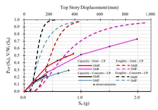
Figure 7. The fragilities and capacities of the model structure as functions of the spectral acceleration (evaluated at T<sub>1</sub>=1.3 seconds) and the roof displacement. Shown for safe-to-fail model Of Steel and concrete, OMFs and SMFs
there were sixteen observation points times eleven records, or 176, iterative computer runs to obtain the median fragilities and capacities, shown in Figure 7. The following observation could be made.
The initial slopes at elastic regimes showed little variations which was consistent with the structural fundamental periods that were in the range of 1.26-1.45 seconds (Tables 2 and 3); the least period (highest slope) for the steel OMF-SM (safe-to-fail model) of 1.26 seconds, the largest one (lowest slope) for the steel SMF-SM of 1.45 seconds, and the intermediate of 1.31 seconds for the concrete safe-tofail structures. The elastic regimes ended with the first yield points (FY) which showed the highest base shear coefficient and spectral acceleration (or top story displacement) for the steel OMF-SM, but the lowest for the concrete SMF-SM model, the steel SMF-SM was the second, and the concrete OMF-SM was the third. These indicated the best elastic behavior for the steel OMF-SM. The conditional probability of collapse, or the fragility, associated with the first yield points is presented in Table 4. The fragilities of the OMF-SM are about twice those of the SMF-SM for their respective first yield points, but lower for steels than those of concretes. Judging from these fragilities alone, it could be stated that the SMFs had lower conditional collapse risks than those of the OMFs at the first yield points. When the capacity values of the FY points are divided by the safety factor (SF=1.6) then the design points are obtained. The conditional probabilities of collapses associated with these points are all 5% (observe Figure 7, lower-left corner).
Similar observation for post-elastic regimes, especially at their ends, could also be performed. The highest capacity at collapse prevention (CP) was shown by the steel SMF-SM model, its ductility was \(\mu\)=5 (the ductility is defined as the displacement at CP divided by that of FY). Consequently, the response modification factor is R = \(\mu\) x SF = 5 x 1.6 = 8; so, this became the ratio between the displacements at the CP to that of the design point. The second highest was indicated by the steel OMF-SM model, with the ductility of \(\mu\)=2.2, much lower than that of the SMF-SM model. Assuming that damage state is affected
mostly by the ductility, at the CP points, the OMF-SM underwent much lower damage state than that of the SMF-SM models. This is also supported by the total drift ratio of 1.4% and 3.1% for OMF-SM and SMF-SM, respectively, for steel. The concrete models exhibited a similar behavior; higher capacity was shown by SMF-SM than by OMF-SM models, but at different ductility ratios of u=5 and 1.88 for SMF-SM and OMF-SM, respectively. The total drifts were 1.3% and 0.7% in the respective order. These clearly showed that the damage state is much more severe for SMF-SM than that of OMF-SM models. Based on the discussions, in general, the steel safe-to-fail models presented superior performance than the concrete counterparts; as also the OMF-SM was preferable than the SMF-SM, due to less severe damage state. Recall that at CP, all models had the conditional probability of collapse prevention of 95% or higher, and at the failure state as shown in Figure 5, but at their respective ductility and total drift ratios.
A more comprehensive understanding could only be observed when the spectral hazard was employed, and the probabilities of collapses were computed and compared. However, more remarks on the fragilities could be made a priori. It would be evident later that their most contributions came from the lower parts of the fragilities, the more right shifted the less their contributions in the probabilities of collapses. Thus, it could be anticipated that the probability of collapse of the concrete would be higher than that of the steel models (observe Figure 7); more surprisingly, the concrete SMF-SM would result in higher probability of collapse than the OMF-SM; similarly, for steel structures (observe Figure 7, lower-left corner).
6. The Probability of Collapse
The probability of collapse is simply the integral of the joint probability density function of the spectral acceleration (as the demand) and the structural capacity as two random variables. Performing the integration for which the capacity is less than or equal to the demand for all possible values of the demand, one can obtain the following expression (e.g., Kennedy and Ravindra, 1984),
\[P_{CP} = \int_{0}^{\infty} H(S_a) \frac{dP_{CP}(S_a)}{dS_a} dS_a \approx \Delta P_{CP} \sum_{i} H(S_{ai}) \leq P_g\] (4)
Where \(P_{CP}\) is the probability of collapse, \(P_{CP}(S_a)\) is the structural fragility at a given \(S_a\), \(H(S_a)\) is the hazard of \(S_a\) (as shown in Figure 1), and \(P_g\) is the performance goal specified by codes. For illustration, the median values of \(P_g\) is \(10^{-5}\) per annum for certain structures, systems, and components of nuclear power plants for the highest safety class (IAEA, 2021). The resulting computations of Eq. (4) were listed in Table 5 for the steel and concrete, OMF-SM and SMF-SM models.
It was observable that only the steel safe-to-fail structures satisfied the required performance goal of 10 <sup>-5</sup> per annum. Of these two, the steel OMF-SM model showed the least probability of collapse, much lower
Table 4. The conditional probability of collapse associated with the first yield points of safe-to-fail models
| D 1 | C | C 50 |
|---|---|---|
| \(P_{CP}\) | \(o_a\) | \(=\) \(S_{a,95}\) FY |
| , , , , | ||
|---|---|---|
| OMF | SMF | |
| Steel | 0.35 | 0.18 |
| Concrete | 0.42 | 0.21 |
Table 5. The probability of collapse of safe-to-fail models (per annum)
| OMF | SMF | |
|---|---|---|
| Steel | 8.29 x 10⁻⁸ | 1.38 x 10⁻⁶ |
| Concrete | 1.42 x 10⁻⁵ | 7.07 x 10⁻⁵ |
Performance goal, \(P_a\)=10<sup>-5</sup> per annum for SDC1-NPPs [IAEA, 2021].
than the performance goal of 10<sup>-5</sup> pa. It had the lowest fundamental period (see Tables 2 and 3) or the stiffest among the four models, it weighed much less than that of the concrete model, and if it ever achieved the collapse prevention (CP) point it would show lower ductility (µ =2.2) and drift ratios (1.4%), indicating low damage state. Certainly, the steel OMF-SM is the model of choice, as it provided wide room for optimization guided by the closeness of the probability of collapse to the performance goal. The second alternative, based on the probability of collapse, was the steel SMF-SM model. It was the most flexible (\(T_1\)=1.45 seconds), it was of comparable weight, but when it ever achieved the CP, it would show the highest ductility (\(\mu\)=5) and drift (3.1%) ratios, and hence, more severe damage state than the former. It provided narrower room for optimization. However, in general, based on the probability of collapse, the damage state and the cost effectiveness, the OMF-SM were preferable than the SMF-SM models.
When the steel OMF-SM model was chosen along with an optimization scenario, some reduction of the structural components could be made. The reduction could be started with beams by stressing that they must remain compact at supports and sufficiently braced to allow for plastic hinges formation. Then move on to columns which should have the SCWB ratio of three-tofour. Columns at the first storey must be compact and well detailed to develop plastic hinges. Iterations should be performed to achieve the optimum probability of collapse, thereby obtaining an efficient, yet reliable, steel OMF-SM model. The detail of the procedure is out of the scope of the present study.
7. Summary
Seismic design and risk analyses of frames for nuclear facilities were discussed based on the state-of-the-art provisions. The frames were of concrete and steel structures, and were designed for strong column-weak beam ratios of 3-4. With these high ratios, it was anticipated that should failure occur it would be that of beam-sway mechanism and no plastic hinges would develop in columns except at their bases and tops. This failure mechanism was expected to be safer, and thereby, referred to as safe-to-fail mode herein. Furthermore, the column detailing could be made minimal for there were no hinges expected in them except at their bottoms and tops. All plastic hinges were designed to form in beams, suggesting them to always have sufficient ductility capacities.
Two types of structures were investigated, i.e., ordinary and special moment frames, abbreviated as OMFs and SMFs. As required by the provisions, they have different detailing/confinement or b/t (sectional slenderness ratio) requirements, being more stringent for SMFs. The ductility demands were different as well, being more than twice for SMFs than that of OMFs. In the design, sectional ductility ratios of about 2 and 5 were used for OMF and SMF beams, respectively. This justifies the lower requirements for OMF beams detailing. Because of lower ductility, and hence the response modification factor, the OMF structures were designed for higher base shear forces. Consequently, they are heavier and tend to be stiffer than SMFs, as also they showed lower probability of collapse in this study.
Four structures of steel and concrete each for safe-tofail OMFs and SMFs were designed and tested for eleven ground motions time series. The spectra of the ground motions were all spectrally matched to the site smooth spectra. Incremental dynamic analyses were performed such that fragility and capacity curves could be constructed for each structure. The spectral acceleration at the structures' fundamental periods was selected as the intensity measure, while the damage measure was the development of beams plastic hinges as many as fifty percent of total potential plastic hinges in the structure. When the damage measure associated with the collapse criterion was reached, the base shear, top story drift, and spectral acceleration were observed.
Comparisons of the four capacity curves showed that, at collapse event, the safe-to-fail steel SMF yielded the highest base shear force or strength, followed by the safe-to-fail steel OMF. The collapse drift as also the ductility ratio was lower for the safe-to-fail steel OMF than that for the safe-to-fail steel SMF, suggesting less severe damage state of the former. Similar observation could be deduced for safe-to-fail concrete structures. However, in this study, in general, the safe-to-fail steel structures were stronger than their concrete counterparts; although, the latter were almost twice heavier than the former.
The probabilities of failure as the convolution of the spectral acceleration hazard and the structural fragility curves were also computed. The safe-to-fail steel OMF produced the least probability of failure followed by the safe-to-fail steel SMF. They both satisfied the code requirement for the target performance goal, which could not be met by the safe-to-fail concrete structures. Judging from the performance, weight and the probability of collapse points of view, the safe-to-fail steel OMF could be considered as a model of choice. The model provided wide enough room for optimization and thereby might raise its cost competitiveness.
8. Conclusions
In concluding the study, the following main points could be produced:
- 1. The safe-to-fail design could only be achieved through high strong-column-weak beam ratio of about 3-4; in which case the failure would be in beam-sway mechanism. The beam failure should be ensured to follow the flexural mode only leaving no room for premature failures.
- 2. The SMF and OMF structures have different requirements on their detailing, being more stringent for SMF than for OMF. This is because the SMF required much higher ductility factor, making it slimmer than the OMF, or, in other words, the OMF was more robust than the SMF. For the same material their weight was comparable, and, in case of the safe-to-fail models, the former tended to show lower probability of collapse and lower damage state than the latter should they fail.
- 3. The study showed that the safe-to-fail steel OMF structures possessed lower probability of collapse than their concrete SMF counterparts in such a way that ample room for optimization was available. The safe-to-fail steel OMF was the model of choice according to the study.
Acknowledgement
The authors acknowledge the support of the Engineering Center for Industry of the Institute of Technology Bandung, and the Research Center for Ecohydrology, Ecohydraulic and Engineering Sciences.