
1 Introduction
In the automobile sector, companies are progressively dedicated to creating a holistic experience for their consumers. Not only do the companies have to keep up with their rivals, but they also have to sustain themselves in the market [1]. For that, industries are in an endless search for improving their products to attract buyers. Therefore, various empirical studies on consumer responses related to product design focused on the relationship among consumers' subjective
responses towards objective features associated with the product [2]. Researchers have tried to measure consumer attitudes or cognitive feelings by presenting a different range of product forms. For the categorization of consumer responses, various theoretical frameworks have been developed related to product design. Thus, product design and its effect on consumer behavior have become a significant area of interest for researchers [3]–[5]. At the same time, consumer satisfaction is an inherently emotional and cognitive response [6]. Consumers want to purchase unique products in contrast with other available products. Nowadays, aesthetics is one of the prime components of everyday products by which consumers and designers are inspired [7]. In this framework, researchers put more stress on the consumer's cognitive thinking rather than the designer's thinking. The consumer's thinking on a product design is different for different components of the product experience: aesthetic pleasure, emotional response, and attribution of meaning. Although the use of aesthetics is an efficient way to separate/distinguish a product (only by seeing them), it also has a significant impact on the customer's perception at the time of purchase [5], [8]. Various companies have tried to distinguish their products by using aesthetics, making them look more efficient and innovative [9]. Various research works in different product design related areas have been carried out, such as visual product aesthetics [10], product form [11], consumer behavior [12], etc. In this study, we tried to identify the non-visual factors that influence the attractiveness of a car. After that, we identified different sub-factors of these non-visual factors and tried to obtain the relationships between these sub-factors.
1.1 Current Status of the Automobile Sector in India
The Indian automobile sector is developing very fast and currently is the fifth largest manufacture in the world, after having been in seventh place in 2017. Presently, the automobile industry contributes more than 7.1% to India's gross domestic product (GDP). For the first three quarters of 2020, auto companies in India manufactured approximately 2.16 million vehicles, down 38.4% compared to the 3.5 million vehicles manufactured during the first three quarters of 2019 [13]. Indian automotive industries directly or indirectly generate employment for 35 million people. The 118-billion-dollar automotive sector is estimated to reach a market of approximately 300-billion-dollar by the end of 2026. India's annual production was 30.91 million vehicles in 2019 against 29.08 million in 2018, registering a healthy growth of 6.26%. Such a drastic growth has created concern for consumer emotional perception and their expected needs from automobile manufacturers [14]. These concerns are not only limited to the designer's perception at the time of designing a new car but also spread across the consumers' emotions and their perception at the time of purchase of a new car, or when planning the purchase of a new car. This difficulty was dealt with by using simple multi-criteria decision-making techniques for finding the top subfactors for non-visual factors in our previous study [5].
1.2 Research Objective
According to Blessing and Chakrabarti [15], the general idea of design research is to make product design 'more efficient and effective' and make products more successful. The objective of this study was threefold: (1) to identify the major non-visual factors related to cars that affect the consumer's purchase behavior and the designer's thinking at the time of designing a new car through previous works; (2) to identify the various sub-factors of the non-visual factors identified through a literature search; (3) to establish and examine the causal relationships between the finalized sub-factors and the top non-visual factors to identify the most significant sub-factors. First, we conducted an extensive literature search to find the top non-visual factors, and then we conducted a survey to find the various sub-factors related to the non-visual factors of cars. After that, the DEMATEL method was used to obtain the causal relationships between sub-factors, which show the type of influence that one sub-factor has on another sub-factor.
A causal relationship is normally validated with the support of a causal diagram that distributes the factors under study into cause-and-effect factors. A cause factor commands some influence on the arrangement and an effect factor receives this command. The Decision-Making Trial and Evaluation Laboratory (DEMATEL) technique was used to develop an interaction matrix that expresses the inter-relationships between the sub-factors of the top non-visual factors. Subfactors that are cause factors and have an inter-relationship with most of the other sub-factors will have a greater possibility to improve the non-visual factors, which will fulfill the consumer's emotional, practical desires.
The rest of this article is organized as follows: In Section 2, we discuss previous research associated with the factors of cars and consumers' and designers' thinking on these factors. The proposed framework was based on an open-ended survey and the DEMATEL method (this work's main methodology) is explained in Section 3. In Section 4, the collection of data for this study is explained. An application of the proposed work is provided in Section 5, which is followed by the conclusions and limitations of this work in the last section.
2 Literature
As we have seen in previous studies, numerous visual factors affect the consumers' cognitive perception. Apart from these visual factors that lead to the failure/success of any segment of automobiles [8], there are some other factors, such as ergonomics, warranty/quality, past experiences, etc. In some
experimental studies, it was observed that the customers had a higher preference for some designs compared to others designs [16], [17], but little seems to be known about how consumers understand product designs and how they can translate them into insights of value [18]. Whereas Orth and Malkewitz [17] concluded in their study that numerous factors affect the consumer's cognitive appeal at the time of purchase. These factors may be visual or non-visual. The judgment may vary from person to person or from product to product, but it is based on visual information and is also often based on the functionality, elegance, and social significance of the product [2]. These decisions often show a connection between the perceived characteristics of the product, and they frequently point towards the consumers' desires rather than their needs [19]. Generally, car buyers expect a car to have a variety of accessories. If these accessories are available, then buyers consider it as a good-quality car. Quality is the perceived performance of a service or product [20]. However, quality itself alone is not enough; whether the product is reliable enough is also important. A product's reliability is usually explained as a reason for consumers to repurchase a specific product or service in the upcoming period [18]–[23]. Other non-visual factors, apart from quality and reliability, eventually lead to the success or failure of any vehicle in the market. This article focuses only on the automobile industry and especially to passenger cars. However, we identified various non-visual factors in our previous research that affect consumer perception while buying a new car [5]. The list of non-visual factors is given in Table 1.
Table 1 List of non-visual factors that influence the purchase of cars [5].
| Status/feeling of prestige | Reliability | New technology/features |
|---|---|---|
| Ergonomics | Quality/warranty | Past experience |
| Safety features | Design/unique form | Mileage/fuel-efficiency |
2.1 Research Gap
The factors that were found are related to the automobile sector, especially for cars and there is a need to explore the sub-factors of each main factor that is mentioned in Section 2. Some researchers have attempted to find out the relations between two or three factors, such as ergonomics and product quality [24], [25], studying the relation of consumer willingness and their preferences to pay for new vehicle technology. We found few relationships between these factors and to date no study has been conducted on what type of sub-factors affect the main non-factors mentioned in Section 2. Therefore, a study should be carried out that does not only show the connection between different sub-factors but can also show the ability of each sub-factor to affect the other sub-factors for the enhancement of main non-visual factors and fulfilling the consumers' needs and desires.
3 Aim and Methodology
This research aimed to find the most prominent set of sub-factors associated with each top non-visual factor, as found in the existing literature [5]. The list of nonvisual factors is given in Section 2 (Table 1). To achieve the above aim, we used the following methodology: (i) first, we reviewed the literature to find out the non-visual factors related to passenger cars, (ii) then we identified the various sub-factors that affect the non-visual factors of a car. For finding the sub-factors, we conducted an open-ended survey among car buyers and prospective car buyers. Among these sub-factors, we found the most prominent factors and their relationships with each other and the non-visual factors. To find the most prominent sub-factors, we used the DEMATEL approach. Even though there are other useful decision-making methods, for example Interpretive Structural Modeling (ISM), Elimination and Choice Expressing Reality (ELECTRE), Analytical Network Process (ANP), etc., these techniques/approaches are only able to prioritize sub-factors/criteria and are unsuccessful in detecting cause-andeffect factors. An understanding of the cause-and-effect factors helps professionals/experts in comprehensive decision-making. A detailed description of the DEMATEL technique is given below.
3.1 The DEMATEL Technique
From 1972 to 1976, the Battelle Memorial Institute of Geneva ran a science and human affairs program for solving interconnected and complex problems and proposed a Decision-Making Trial and Evaluation Laboratory [26]. For comprehensive decision-making, the DEMATEL technique is beneficial for experts from all industries. It is based on digraphs and is used not only to find the inter-relationships between sub-factors/criteria, but also helps in finding the direction of these relationships [27]–[29]. The key points of the DEMATEL approach are: (a) it is based on graph theory and simplifies the analysis of challenging problems with the help of visualization; (b) it helps to develop the cause-and-effect relationships among different sub-factors/criteria, which makes it easy to understand the mutual impact of these factors/sub-factors/criteria, and (c) with this method, we can find out the strength of the relationships among different factors, which is impossible with other multi-criteria decision-making techniques [30]. This method has broadly been applied in different areas, such as online reputation management [31], identification of critical factors for green supply chain management [32], sustainable supply chain [33], sustainable food supply chain [27], and logistics management implementation [34]. This approach/technique does not require large amounts of data.
The steps of the DEMATEL technique are:
- 1. Construction of an initial relational matrix. In the first step, an initial relational matrix is constructed for the sub-factors with professionals/experts' help. The views of the experts/professionals are collected using the linguistic rating scale shown in Table 5.
- 2. Construction of a direct-relation (average) matrix. The average direct-relation matrix is generated from the initial relation matrix. We asked the experts to score each sub-factor, according to which they believe a sub-factor i influences sub-factor j using a comparison scale. The notion \(x_{i,j}^k\) specifies the extent to which according to expert's k judgment sub-factor i influences sub-factor j. The experts use the non-negative numbers in Table 5. The variables \(X^1, X^2, X^3, \cdots, X^L\) are the inputs of each expert that create a \(n \times n\)-sized non-negative matrix \(X^k = \left[x_{i,j}^k\right]_{n \times n}\) for \(k \in [1, L]\). There is no influence from the sub-factors, so each matrix's diagonal element is zero. To integrate all opinions from L experts, the average matrix \(A = \left[a_{i,j}\right]\) can be constructed as follows:
\[[a_{i,j}] = \frac{1}{L} \sum_{k=1}^{L} [x_{i,j}^k]\] (1)
3. Construct a normalized direct-relation matrix. Based on the average direct-relation matrix (A), a normalized initial direct relation matrix (N) can be obtained by N = AP, with
\[P = \min \left\{ \frac{1}{\max i \sum_{i=1}^{n} a_{i,j}}, \frac{1}{\max j \sum_{j=1}^{n} a_{i,j}} \right\}\] (2)
where \(0 < n_{i,j} < 1\). Similarly, a positive scalar P takes the largest of the two factors, and the matrix N is calculated by dividing each element of matrix A with the positive scalar P.
4. Calculate a total-relation matrix (T). Once the normalized direct relation matrix (N) has been obtained, the total relationship matrix \(T_{n\times n}\) is obtained as follows:
\[T = N(I - N)^{-1} (3)\] where I is the identity matrix.
5. Formation of a causal diagram. The sum of rows and the sum of columns are separately denoted as vectors r and c within the total relation matrix T, respectively. In the total relation matrix, the sums of rows r and columns c are computed as r and c, \(n \times 1\), and \(1 \times n\) vector, as shown below:
\[r = \left(\sum_{j=1}^{n} t_{i,j}\right)_{n \times 1} \tag{4}\]
\[c = \left(\sum_{i=1}^{n} t_{i,j}\right)_{1 \times n} \tag{5}\]
The casual diagram is prepared by mapping prominence + and relation − data, marked horizontally and vertically in the graph. Then the categorization of sub-factors into cause or effect group is done. If the − value is positive, sub-factors come in the cause group, and if the − value is negative, they come in the effect group. The + value indicates the importance level of the factor and r – c indicates a causeand-effect factor.
6. Construction of an interaction matrix of sub-factors. The average of the elements in the total relation matrix gives the threshold value, since matrix provides instances of how one sub-factor affects another. Thus, the threshold value assists in filtering out some insignificant/negligible effects in this context. Further, the results that are greater than the threshold value will be selected, as shown in the interaction matrix of sub-factors.
3.2 Finding Sub-factors for Non-visual Factors
At least five experts should be involved in a study that is based on decisionmaking [35]. For the collection of sub-factors, we conducted an open-ended survey. We made a questionnaire related to non-visual factors of cars, which can be found in Appendix 1. During the open-ended survey, we asked eighteen experienced car owners to provide their responses to each question. All the participants were male, their average age was thirty-two years, and they had different social, economic, and cultural backgrounds. Despite having eighteen respondents, we only received a response from fifteen respondents; the other three left the survey in the middle due to time and work constraints. Therefore, we eliminated these three incomplete replies from the final cumulative collection. Out of fifteen car owners, six worked in different multinational companies, and the rest worked as senior research associates. All of them had two to four years of industrial experience, and all of them had more than six to seven years of car driving experience.
Each respondent took approximately forty-five minutes to complete the survey. Each respondent mentioned a respective sub-factor for each non-visual factor on a priority basis; the entire list is presented in Appendix 2. In Table 10 of Appendix 2, the first respondent listed 'safety' as the first priority as a sub-factor of reliability; the second respondent listed 'airbag, brand values, seat locking system, and brake system' as the first priority under the same factor. In the next
step, we listed all the sub-factors for each non-visual factor mentioned by all respondents, and then added all of them.
3.3 Grouping of Sub-factors
We obtained various sub-factors from the respondents for every non-visual factor. Next, we used the English dictionary, blogs (websites), and technical books related to car/vehicles to find out synonyms for each sub-factor. Then all words with a similar meaning were grouped together and one representative name was selected. As we saw in Appendix 2, the sub-factors other than the top five (six, seventh, and so on) got the same level of priority. Then, we took the top five sub-factors for each non-visual factor, which are listed in Table 2.
| Table 2 | List of sub-factors according to their respective non-visual factors |
|---|---|
| (frequency of occurrence in brackets). |
| Unique form/design | Feeling of prestige/status | Quality | Ergonomics | Reliability | Safety | Mileage/fuel- efficient | New technology/ features | Past experience |
|---|---|---|---|---|---|---|---|---|
| Design of head/ taillights (6) | Brand value (6) | Car build quality (9) | Adjustable seat, steering & mirror (8) | Good engine performance (6) | Airbags (10) | Weight of the car (6) | Cost (8) | Engine performance/ mileage (6) |
| Design & looks of the car (4) | Design & looks of the car (6) | Safety (3) | Leg/inside space (8) | Regular car servicing (5) | ABS (7) | Eco-mode feature (5) | New features improving safety (6) New | Car servicing (6) |
| Aerodynamic look (3) | Comfort (4) | New accessories/ features (3) | Comfortable seat size & design (6) | Safety (4) | Car build quality (7) | Engine performance (5) | technology enhancing engine performance (3) | Comfort (4) |
| Height & ground clearance (2) | High-end features & interior (4) | Reliability (3) | Height & ground clearance (4) | Brand value (4) | Height & ground clearance (5) | Aerodynamics of the car (4) | New smart features (2) | Brand value (3) |
| Inside space (2) | Good engine performance (3) | Good engine performance (3) | Cost (2) | Car build quality (4) | Cost (2) | Proper car servicing (2) | New features increase comfort level (2) | Sitting space (3) |
In Table 2, we present the various sub-factors under each category (main non-visual factors) in descending order of frequency. For instance, we can see that the main non-visual factor 'reliability' is affected by the sub-factors 'good engine performance (6)', 'brand value (4)', 'build quality (4)', 'proper car servicing (5)', and 'safety (4)' in decreasing order, and so on for the other non-visual factors. The numeric value represents the different respondents who chose one particular sub-factor for that particular rank/preference during the open-ended survey.
After, collection of the different sub-factors we wanted to find the relationships between the sub-factors and the main factors, since the number of sub-factors was very high. The reason was that there was repetition of sub-factors, as we can see in Table 2. The respondents considered 'safety of the car' as a sub-factor for the main factors 'quality', 'reliability' as well as 'new technology/features', as shown in Figure 1.
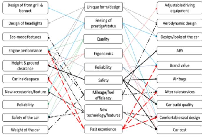
Figure 1 Relationship between the main factors and their sub-factors.
Similarly, there were other factors too, which were considered sub-factors for other main non-visual factors. Figure 1 shows how one sub-factor is linked with different main non-visual factors. With the help of Figure 1 we could identify 20 sub-factors that affect the top nine non-visual factors. After finding the twenty different sub-factors, it was necessary to identify the most prominent sub-factors among them, which are given in Table 3.
Table 3 List of all sub-factors obtained after finding the similarity between them.
| No. | Sub-factor | No. | Sub-factor | No. | Sub-factor | No. | Sub-factor |
|---|---|---|---|---|---|---|---|
| F1 | Adjustable driving equipment | F6 | After-sale services | F11 | Design of front grill & bonnet | F16 | Car inside space |
| F2 | Aerodynamic design | F7 | Car build quality | F12 | Design of headlights | F17 | New accessories/f eature |
| F3 | Air-bags | F8 | Comfortable seat design | F13 | Eco-mode feature | F18 | Reliability |
| F4 | ABS | F9 | Car cost | F14 | Engine performance | F19 | Safety of the car |
| F5 | Brand value | F10 | Design/looks of the car | F15 | Ground clearance | F20 | Weight of the car |
Note: F1 denotes the sub-factor 'adjustable driving equipment,' F2 denotes the sub-factor 'aerodynamic design', and so on until F20.
4 Data Collection and Results Analysis
We conducted an open-ended survey to find out the sub-factors of each nonvisual factor among prospective car buyers, i.e., people who are thinking to purchase a car the coming year. Next, we used a decision-making technique for prioritization, i.e., the DEMATEL technique, and to identify the influence of each sub-factor on the main non-visual factors. The DEMATEL approach was used to understand the inter-relationships between the sub-factors and also to recognize the cause-and-effect factors by developing a causal diagram.
After the collection of the sub-factors, they were arranged in matrix form, as depicted in Appendix 3. We approached six automobile designers/professionals to obtain their views on each sub-factor with respect to the others and requested them to give their response by using the comparison scale in Table 4. All six designers had at least eight years of industrial experience, and currently worked in multinational automobile companies. During this study, experienced people played an important role. As mentioned in Section 3.2, the minimum number of experienced professionals required is five [35].
Numeral Definition 0 No influence 1 Low influence 2 Medium influence 3 High influence 4 Very high influence
Table 4 Linguistic approach for the DEMATEL method.
The expert input is presented in the form of an initial relation-matrix, provided in Table 11, Appendix 4. The input of one expert is provided as an example in Table 12, Appendix 4. After that, by using Equation (1), the inputs of all six are experts were aggregated, as shown in Table 5).
Table 5 was obtained by averaging the inputs of the six experts. For instance, in the third row and the fifth column of Table 5, the value 0.17 shows an average input of 1 = 0,2 = 1,3 = 0,4 = 0,5 = 0,6 = 0, where denotes 'experts/professional designers'. After calculating the direct relation average matrix, the normalized direct relation matrix was developed for the twenty subfactors by using Equation (2), as provided in Table 6.
| * | F1 | F2 | F3 | F4 | F5 | F6 | F7 | F8 | F9 | F10 | F11 | F12 | F13 | F14 | F15 | F16 | F17 | F18 | F19 | F20 |
|---|---|---|---|---|---|---|---|---|---|---|---|---|---|---|---|---|---|---|---|---|
| F1 | 0.00 | 0.33 | 1.67 | 0.17 | 3.33 | 0.67 | 1.17 | 3.33 | 2.83 | 2.67 | 0.00 | 0.00 | 0.33 | 0.00 | 0.00 | 2.00 | 1.50 | 2.00 | 2.83 | 1.00 |
| F2 | 0.00 | 0.00 | 0.00 | 0.17 | 1.00 | 0.17 | 2.17 | 1.83 | 1.50 | 3.00 | 3.00 | 2.00 | 0.33 | 1.33 | 1.83 | 0.50 | 0.50 | 0.67 | 1.67 | 1.17 |
| F3 | 2.00 | 0.50 | 0.00 | 0.00 | 3.50 | 0.67 | 1.00 | 1.00 | 2.83 | 1.00 | 0.00 | 0.00 | 0.00 | 0.00 | 0.00 | 0.67 | 1.33 | 2.00 | 3.67 | 0.67 |
| F4 | 0.50 | 0.33 | 0.00 | 0.00 | 2.83 | 1.67 | 1.17 | 2.00 | 2.83 | 0.00 | 0.00 | 0.00 | 0.17 | 0.67 | 0.17 | 0.00 | 1.00 | 2.33 | 3.67 | 0.50 |
| F5 | 2.33 | 1.83 | 3.00 | 2.67 | 0.00 | 2.00 | 2.67 | 2.50 | 2.67 | 2.50 | 1.83 | 2.17 | 2.00 | 1.50 | 1.00 | 1.33 | 2.50 | 2.67 | 3.00 | 1.50 |
| F6 | 1.00 | 0.17 | 0.67 | 1.17 | 2.33 | 0.00 | 0.67 | 1.50 | 2.67 | 0.33 | 0.33 | 0.00 | 0.83 | 2.00 | 0.00 | 0.17 | 0.17 | 1.83 | 2.50 | 0.50 |
| F7 | 0.83 | 0.83 | 0.50 | 0.67 | 2.67 | 0.67 | 0.00 | 2.67 | 2.83 | 2.33 | 1.67 | 1.50 | 1.33 | 0.50 | 0.50 | 0.83 | 0.83 | 2.67 | 3.50 | 2.17 |
| F8 | 3.00 | 1.00 | 0.83 | 2.00 | 2.83 | 1.83 | 2.67 | 0.00 | 2.83 | 1.00 | 0.50 | 0.33 | 2.00 | 1.33 | 0.83 | 1.50 | 1.00 | 2.17 | 2.33 | 1.67 |
| F9 | 2.17 | 1.67 | 2.33 | 2.33 | 2.33 | 2.00 | 3.00 | 2.83 | 0.00 | 2.67 | 2.50 | 2.67 | 2.33 | 2.00 | 0.67 | 1.50 | 2.50 | 2.83 | 3.33 | 1.33 |
| F10 | 1.50 | 2.33 | 0.33 | 0.00 | 2.33 | 0.67 | 2.17 | 1.50 | 3.17 | 0.00 | 3.50 | 3.33 | 0.00 | 0.00 | 2.33 | 1.83 | 2.00 | 1.67 | 1.67 | 2.00 |
| F11 | 0.00 | 2.67 | 0.00 | 0.00 | 1.67 | 0.00 | 1.17 | 0.17 | 2.50 | 3.67 | 0.00 | 1.00 | 0.00 | 0.33 | 0.50 | 0.00 | 0.33 | 1.83 | 1.00 | 1.00 |
| F12 | 0.00 | 2.00 | 0.00 | 0.33 | 1.50 | 0.00 | 1.17 | 0.17 | 2.50 | 3.00 | 1.17 | 0.00 | 0.00 | 0.00 | 0.50 | 0.00 | 0.00 | 0.83 | 1.00 | 0.50 |
| F13 | 0.00 | 1.00 | 0.33 | 0.50 | 2.00 | 0.50 | 4.00 | 1.50 | 2.17 | 0.67 | 0.00 | 0.00 | 0.00 | 3.17 | 0.00 | 0.00 | 1.50 | 1.67 | 1.17 | 0.33 |
| F14 | 0.00 | 1.50 | 0.00 | 0.33 | 2.33 | 2.50 | 1.50 | 1.33 | 2.50 | 0.33 | 0.83 | 0.00 | 2.83 | 0.00 | 0.17 | 0.00 | 0.33 | 2.33 | 2.17 | 1.33 |
| F15 | 0.00 | 2.33 | 0.00 | 0.17 | 1.17 | 0.33 | 1.00 | 1.00 | 0.67 | 1.83 | 0.67 | 0.50 | 0.00 | 0.17 | 0.00 | 0.50 | 0.17 | 1.83 | 2.33 | 1.67 |
| F16 | 1.83 | 1.00 | 0.67 | 0.00 | 0.83 | 0.50 | 1.17 | 2.17 | 2.50 | 2.33 | 0.33 | 0.00 | 0.00 | 0.00 | 0.67 | 0.00 | 1.83 | 1.00 | 1.50 | 1.17 |
| F17 | 1.67 | 0.50 | 1.17 | 1.00 | 1.83 | 1.17 | 1.00 | 1.67 | 3.00 | 2.50 | 1.67 | 0.67 | 2.00 | 0.33 | 0.17 | 1.83 | 0.00 | 1.00 | 2.33 | 1.00 |
| F18 | 2.50 | 0.83 | 2.50 | 2.67 | 2.83 | 1.50 | 2.83 | 2.67 | 2.33 | 1.83 | 1.33 | 1.33 | 1.67 | 2.00 | 1.33 | 2.17 | 2.17 | 0.00 | 2.83 | 1.00 |
| F19 | 2.67 | 1.50 | 3.67 | 3.50 | 2.50 | 2.33 | 3.00 | 2.33 | 3.33 | 1.00 | 1.67 | 1.00 | 0.17 | 1.67 | 1.00 | 1.00 | 1.17 | 2.50 | 0.00 | 2.00 |
| F20 | 0.83 | 1.17 | 0.50 | 0.67 | 1.50 | 0.17 | 1.67 | 1.17 | 2.33 | 2.00 | 1.50 | 0.50 | 0.33 | 1.17 | 0.83 | 0.67 | 1.17 | 1.67 | 2.17 | 0.00 |
Table 5 Linguistic approach for the DEMATEL method.
Note: F1 (Adjustable driving equipment), F2 (Aerodynamic design), F3 (ABS), F4 (Air-bags), F5 (Brand value), F6 (After-sale services), F7 (Car's build quality), F8 (Comfortable seat design), F9 (Car cost), F10 (Design/looks of the car), F11 (Design of front grill & bonnet), F12 (Design of headlights), F13 (Eco-mode feature), F14 (Engine performance), F15 (Ground clearance), F16 (Car inside space), F17 (New accessories/feature), F18 (Reliability), F19 (Safety of the car), F20 (Weight of the car).
Table 6 Normalized Direct-Relation matrix for sub-factors.
| * | F1 | F2 | F3 | F4 | F5 | F6 | F7 | F8 | F9 | F10 | F11 | F12 | F13 | F14 | F15 | F16 | F17 | F18 | F19 | F20 |
|---|---|---|---|---|---|---|---|---|---|---|---|---|---|---|---|---|---|---|---|---|
| F1 | 0.00 | 0.01 | 0.03 | 0.00 | 0.07 | 0.01 | 0.02 | 0.07 | 0.06 | 0.06 | 0.00 | 0.00 | 0.01 | 0.00 | 0.00 | 0.04 | 0.03 | 0.04 | 0.06 | 0.02 |
| F2 | 0.00 | 0.00 | 0.00 | 0.00 | 0.02 | 0.00 | 0.05 | 0.04 | 0.03 | 0.06 | 0.06 | 0.04 | 0.01 | 0.03 | 0.04 | 0.01 | 0.01 | 0.01 | 0.03 | 0.02 |
| F3 | 0.04 | 0.01 | 0.00 | 0.00 | 0.07 | 0.01 | 0.02 | 0.02 | 0.06 | 0.02 | 0.00 | 0.00 | 0.00 | 0.00 | 0.00 | 0.01 | 0.03 | 0.04 | 0.08 | 0.01 |
| F4 | 0.01 | 0.01 | 0.00 | 0.00 | 0.06 | 0.03 | 0.02 | 0.04 | 0.06 | 0.00 | 0.00 | 0.00 | 0.00 | 0.01 | 0.00 | 0.00 | 0.02 | 0.05 | 0.08 | 0.01 |
| F5 | 0.05 | 0.04 | 0.06 | 0.06 | 0.00 | 0.04 | 0.06 | 0.05 | 0.06 | 0.05 | 0.04 | 0.05 | 0.04 | 0.03 | 0.02 | 0.03 | 0.05 | 0.06 | 0.06 | 0.03 |
| F6 | 0.02 | 0.00 | 0.01 | 0.02 | 0.05 | 0.00 | 0.01 | 0.03 | 0.06 | 0.01 | 0.01 | 0.00 | 0.02 | 0.04 | 0.00 | 0.00 | 0.00 | 0.04 | 0.05 | 0.01 |
| F7 | 0.02 | 0.02 | 0.01 | 0.01 | 0.06 | 0.01 | 0.00 | 0.06 | 0.06 | 0.05 | 0.03 | 0.03 | 0.03 | 0.01 | 0.01 | 0.02 | 0.02 | 0.06 | 0.07 | 0.05 |
| F8 | 0.06 | 0.02 | 0.02 | 0.04 | 0.06 | 0.04 | 0.06 | 0.00 | 0.06 | 0.02 | 0.01 | 0.01 | 0.04 | 0.03 | 0.02 | 0.03 | 0.02 | 0.05 | 0.05 | 0.03 |
| F9 | 0.05 | 0.03 | 0.05 | 0.05 | 0.05 | 0.04 | 0.06 | 0.06 | 0.00 | 0.06 | 0.05 | 0.06 | 0.05 | 0.04 | 0.01 | 0.03 | 0.05 | 0.06 | 0.07 | 0.03 |
| \(\mathbf{F}_{10}\) | 0.03 | 0.05 | 0.01 | 0.00 | 0.05 | 0.01 | 0.05 | 0.03 | 0.07 | 0.00 | 0.07 | 0.07 | 0.00 | 0.00 | 0.05 | 0.04 | 0.04 | 0.03 | 0.03 | 0.04 |
|---|---|---|---|---|---|---|---|---|---|---|---|---|---|---|---|---|---|---|---|---|
| F11 | 0.00 | 0.06 | 0.00 | 0.00 | 0.03 | 0.00 | 0.02 | 0.00 | 0.05 | 0.08 | 0.00 | 0.02 | 0.00 | 0.01 | 0.01 | 0.00 | 0.01 | 0.04 | 0.02 | 0.02 |
| \(\mathbf{F}_{12}\) | 0.00 | 0.04 | 0.00 | 0.01 | 0.03 | 0.00 | 0.02 | 0.00 | 0.05 | 0.06 | 0.02 | 0.00 | 0.00 | 0.00 | 0.01 | 0.00 | 0.00 | 0.02 | 0.02 | 0.01 |
| \(\mathbf{F}_{13}\) | 0.00 | 0.02 | 0.01 | 0.01 | 0.04 | 0.01 | 0.08 | 0.03 | 0.05 | 0.01 | 0.00 | 0.00 | 0.00 | 0.07 | 0.00 | 0.00 | 0.03 | 0.03 | 0.02 | 0.01 |
| \(\mathbf{F}_{14}\) | 0.00 | 0.03 | 0.00 | 0.01 | 0.05 | 0.05 | 0.03 | 0.03 | 0.05 | 0.01 | 0.02 | 0.00 | 0.06 | 0.00 | 0.00 | 0.00 | 0.01 | 0.05 | 0.05 | 0.03 |
| \(\mathbf{F}_{15}\) | 0.00 | 0.05 | 0.00 | 0.00 | 0.02 | 0.01 | 0.02 | 0.02 | 0.01 | 0.04 | 0.01 | 0.01 | 0.00 | 0.00 | 0.00 | 0.01 | 0.00 | 0.04 | 0.05 | 0.03 |
| \(\mathbf{F}_{16}\) | 0.04 | 0.02 | 0.01 | 0.00 | 0.02 | 0.01 | 0.02 | 0.05 | 0.05 | 0.05 | 0.01 | 0.00 | 0.00 | 0.00 | 0.01 | 0.00 | 0.04 | 0.02 | 0.03 | 0.02 |
| \(\mathbf{F}_{17}\) | 0.03 | 0.01 | 0.02 | 0.02 | 0.04 | 0.02 | 0.02 | 0.03 | 0.06 | 0.05 | 0.03 | 0.01 | 0.04 | 0.01 | 0.00 | 0.04 | 0.00 | 0.02 | 0.05 | 0.02 |
| \(\mathbf{F_{18}}\) | 0.05 | 0.02 | 0.05 | 0.06 | 0.06 | 0.03 | 0.06 | 0.06 | 0.05 | 0.04 | 0.03 | 0.03 | 0.03 | 0.04 | 0.03 | 0.05 | 0.05 | 0.00 | 0.06 | 0.02 |
| F19 | 0.06 | 0.03 | 0.08 | 0.07 | 0.05 | 0.05 | 0.06 | 0.05 | 0.07 | 0.02 | 0.03 | 0.02 | 0.00 | 0.03 | 0.02 | 0.02 | 0.02 | 0.05 | 0.00 | 0.04 |
| \(\mathbf{F}_{20}\) | 0.02 | 0.02 | 0.01 | 0.01 | 0.03 | 0.00 | 0.03 | 0.02 | 0.05 | 0.04 | 0.03 | 0.01 | 0.01 | 0.02 | 0.02 | 0.01 | 0.02 | 0.03 | 0.05 | 0.00 |
First, we calculated scalar value P using Equation (2):
\[P = \min\left\{\frac{1}{\max i \sum_{i=1}^{n} a_{i,j}}, \frac{1}{\max j \sum_{j=1}^{n} a_{i,j}}\right\} = \left\{\frac{1}{48}, \frac{1}{43}\right\} = 0.0208333\]
Next, P = 0.0208333 was multiplied with each element of the average relations matrix (A) in Table 5 to obtain the normalized relation matrix (N) of Table 6. As can be seen, the sum of each column of the normalized relation matrix was greater than zero and less than one. This proves the feasibility of the DEMATEL technique for this study. After calculating the normalized matrix (N), we computed the total relationship matrix in Table 7 by using Equation (3).
Table 7 Total relationship matrix.
| * | F1 | F2 | F3 | F4 | F5 | F6 | F7 | Fs | F9 | F10 | F11 | F12 | F13 | F14 | F15 | F16 | F17 | F18 | F19 | F20 |
|---|---|---|---|---|---|---|---|---|---|---|---|---|---|---|---|---|---|---|---|---|
| F1 | 0.05 | 0.04 | 0.07 | 0.04 | 0.13 | 0.05 | 0.08 | 0.12 | 0.13 | 0.11 | 0.04 | 0.03 | 0.04 | 0.03 | 0.02 | 0.07 | 0.07 | 0.10 | 0.13 | 0.06 |
| \(\mathbf{F}_2\) | 0.03 | 0.03 | 0.02 | 0.03 | 0.07 | 0.03 | 0.09 | 0.08 | 0.09 | 0.11 | 0.09 | 0.07 | 0.03 | 0.05 | 0.06 | 0.03 | 0.04 | 0.06 | 0.09 | 0.05 |
| \(\mathbf{F}_3\) | 0.08 | 0.04 | 0.04 | 0.04 | 0.12 | 0.04 | 0.07 | 0.07 | 0.12 | 0.07 | 0.03 | 0.03 | 0.03 | 0.03 | 0.02 | 0.04 | 0.06 | 0.09 | 0.13 | 0.05 |
| \(\mathbf{F_4}\) | 0.05 | 0.03 | 0.03 | 0.04 | 0.11 | 0.07 | 0.07 | 0.09 | 0.12 | 0.04 | 0.03 | 0.03 | 0.03 | 0.04 | 0.02 | 0.02 | 0.05 | 0.09 | 0.13 | 0.04 |
| \(\mathbf{F}_5\) | 0.11 | 0.09 | 0.11 | 0.10 | 0.09 | 0.09 | 0.14 | 0.13 | 0.16 | 0.13 | 0.09 | 0.09 | 0.08 | 0.07 | 0.05 | 0.07 | 0.10 | 0.13 | 0.16 | 0.08 |
| \(\mathbf{F_6}\) | 0.05 | 0.03 | 0.04 | 0.05 | 0.10 | 0.03 | 0.06 | 0.07 | 0.11 | 0.04 | 0.03 | 0.02 | 0.04 | 0.07 | 0.02 | 0.03 | 0.03 | 0.08 | 0.10 | 0.04 |
| \(\mathbf{F}_{7}\) | 0.06 | 0.06 | 0.05 | 0.06 | 0.12 | 0.05 | 0.07 | 0.11 | 0.14 | 0.11 | 0.08 | 0.07 | 0.06 | 0.05 | 0.04 | 0.05 | 0.06 | 0.12 | 0.14 | 0.08 |
| \(\mathbf{F_8}\) | 0.11 | 0.06 | 0.06 | 0.08 | 0.13 | 0.08 | 0.12 | 0.07 | 0.14 | 0.08 | 0.05 | 0.04 | 0.07 | 0.06 | 0.04 | 0.06 | 0.07 | 0.11 | 0.13 | 0.08 |
| F9 | 0.10 | 0.09 | 0.10 | 0.10 | 0.14 | 0.09 | 0.14 | 0.14 | 0.11 | 0.13 | 0.11 | 0.10 | 0.09 | 0.08 | 0.05 | 0.07 | 0.10 | 0.14 | 0.17 | 0.08 |
| \(\mathbf{F}_{10}\) | 0.07 | 0.09 | 0.04 | 0.04 | 0.11 | 0.05 | 0.11 | 0.09 | 0.14 | 0.07 | 0.12 | 0.11 | 0.03 | 0.03 | 0.07 | 0.07 | 0.08 | 0.09 | 0.11 | 0.08 |
| \(\mathbf{F}_{11}\) | 0.03 | 0.08 | 0.02 | 0.02 | 0.08 | 0.02 | 0.06 | 0.04 | 0.10 | 0.11 | 0.03 | 0.05 | 0.02 | 0.03 | 0.03 | 0.02 | 0.03 | 0.07 | 0.07 | 0.05 |
| \(\mathbf{F}_{12}\) | 0.02 | 0.06 | 0.02 | 0.03 | 0.06 | 0.02 | 0.06 | 0.03 | 0.09 | 0.09 | 0.05 | 0.02 | 0.02 | 0.02 | 0.03 | 0.02 | 0.02 | 0.05 | 0.06 | 0.03 |
| \(\mathbf{F}_{13}\) | 0.03 | 0.05 | 0.03 | 0.04 | 0.09 | 0.04 | 0.13 | 0.07 | 0.10 | 0.05 | 0.03 | 0.03 | 0.03 | 0.09 | 0.02 | 0.02 | 0.06 | 0.08 | 0.08 | 0.04 |
| \(\mathbf{F}_{14}\) | 0.03 | 0.06 | 0.03 | 0.04 | 0.10 | 0.08 | 0.08 | 0.07 | 0.11 | 0.05 | 0.05 | 0.03 | 0.08 | 0.03 | 0.02 | 0.02 | 0.04 | 0.09 | 0.10 | 0.06 |
| \(\mathbf{F}_{15}\) | 0.03 | 0.07 | 0.02 | 0.03 | 0.06 | 0.03 | 0.06 | 0.05 | 0.06 | 0.07 | 0.04 | 0.03 | 0.02 | 0.02 | 0.02 | 0.03 | 0.03 | 0.07 | 0.09 | 0.06 |
| \(\mathbf{F}_{16}\) | 0.07 | 0.05 | 0.04 | 0.03 | 0.06 | 0.03 | 0.07 | 0.08 | 0.10 | 0.09 | 0.04 | 0.03 | 0.02 | 0.02 | 0.03 | 0.02 | 0.07 | 0.06 | 0.08 | 0.05 |
| F17 | 0.07 | 0.05 | 0.06 | 0.05 | 0.10 | 0.06 | 0.08 | 0.09 | 0.13 | 0.10 | 0.07 | 0.04 | 0.07 | 0.04 | 0.02 | 0.07 | 0.04 | 0.08 | 0.11 | 0.06 |
|---|---|---|---|---|---|---|---|---|---|---|---|---|---|---|---|---|---|---|---|---|
| \(\mathbf{F}_{18}\) | 0.11 | 0.07 | 0.10 | 0.10 | 0.14 | 0.08 | 0.13 | 0.13 | 0.15 | 0.11 | 0.08 | 0.07 | 0.07 | 0.08 | 0.05 | 0.08 | 0.09 | 0.08 | 0.15 | 0.07 |
| F19 | 0.11 | 0.08 | 0.12 | 0.12 | 0.14 | 0.09 | 0.13 | 0.12 | 0.16 | 0.09 | 0.08 | 0.06 | 0.04 | 0.07 | 0.05 | 0.06 | 0.07 | 0.13 | 0.10 | 0.09 |
| \(\mathbf{F}_{20}\) | 0.05 | 0.05 | 0.04 | 0.04 | 0.08 | 0.03 | 0.08 | 0.07 | 0.11 | 0.09 | 0.06 | 0.04 | 0.03 | 0.05 | 0.04 | 0.04 | 0.05 | 0.08 | 0.10 | 0.03 |
Meanwhile, from the matrix \(T_{n\times n}\), we could see how each sub-factor affects other sub-factors. In Equation (3), 'I' denotes an identity matrix. In the next step, with the help of Equations (4) and (5), we computed the sum of rows \([r_i]_{n\times 1}\) as well as the sum of columns \([c_i]_{n\times 1}\) of the total inter-relation matrix \(T_{n\times n}\) to find the 'prominence' and 'relation' value of each sub-factor. The sum of every row and column is given in Table 8. In the meantime, during the calculation of the sum of rows \(([r_i]_{n\times 1})\) and columns \(([c_i]_{n\times 1})\), we also computed the values of \((r_i - c_j)\) and \((r_i - c_j)\) as shown in Table 8.
Table 8 Direct and indirect influence.
| Sub-factors | R | с | r-c | r+c |
|---|---|---|---|---|
| F1 | 1.430 | 1.267 | 0.163 | 2.697 |
| \(F_2\) | 1.141 | 1.183 | -0.042 | 2.325 |
| F3 | 1.194 | 1.065 | 0.128 | 2.259 |
| \(F_4\) | 1.132 | 1.071 | 0.061 | 2.202 |
| F5 | 2.076 | 2.060 | 0.016 | 4.136 |
| \(F_6\) | 1.044 | 1.046 | -0.003 | 2.090 |
| \(F_7\) | 1.565 | 1.820 | -0.255 | 3.385 |
| \(F_8\) | 1.642 | 1.724 | -0.082 | 3.366 |
| F9 | 2.136 | 2.367 | -0.232 | 4.503 |
| \(F_{10}\) | 1.608 | 1.728 | -0.120 | 3.336 |
| F11 | 0.966 | 1.220 | -0.254 | 2.186 |
| F12 | 0.799 | 0.974 | -0.175 | 1.774 |
| \(F_{13}\) | 1.112 | 0.887 | 0.225 | 1.999 |
| \(F_{14}\) | 1.189 | 0.958 | 0.231 | 2.147 |
| F15 | 0.864 | 0.678 | 0.187 | 1.542 |
| \(F_{16}\) | 1.049 | 0.906 | 0.143 | 1.956 |
| \(\mathbf{F}_{17}\) | 1.378 | 1.180 | 0.198 | 2.557 |
| \(F_{18}\) | 1.930 | 1.805 | 0.125 | 3.735 |
| \(F_{19}\) | 1.916 | 2.222 | -0.306 | 4.139 |
| F20 | 1.164 | 1.174 | -0.009 | 2.338 |
Note: adjustable driving equipment, aerodynamic design, airbags, ABS, weight of the car are subfactors.
In Table 8, 'r' and 'c' represent the sum of rows and columns, respectively, while '\((r_i + c_j)\)' shows the degree of significance the factor i has in the system. Also, \(r_i - c_j\) shows the gross effect that factor i has on the system. With the help of mapping the values of r + c as well as r - c, a cause-and-effect diagram was
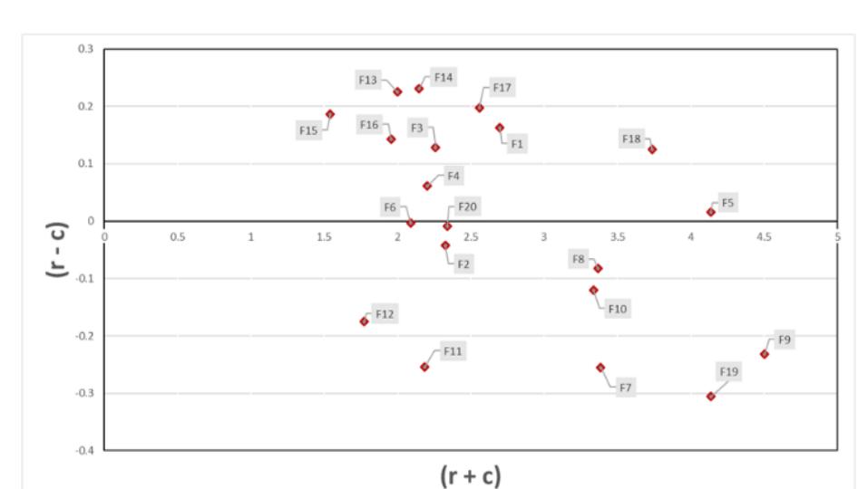
constructed, which is shown below in Figure 2. The horizontal line shows the value of + and the line in the vertical direction shows − .
Figure 2 Digraph showing casual relations among the twenty criteria (subfactors).
After finding the + and − values, it was necessary to filter out some insignificant/negligible effects. For this, decision-makers have to set up a threshold value by using the and values. The interaction matrix was constructed based on a calculated threshold value to give the mutual degree of interaction among the considered sub-factors, as shown in Table 9. The threshold value (i.e., = 0.0683) was obtained by calculating the average of the elements of total relation matrix T. By using this value, we chose only values that were greater than the threshold value. When ( = ), the sum of − is known as 'prominence', which indicates the total effects both received and given by factor . Similarly, the digraph can be attained by using the dataset of + and − .
| * | F1 | F2 | F3 | F4 | F5 | F6 | F7 | F8 | F9 | F10 | F11 | F12 | F13 | F14 | F15 | F16 | F17 | F18 | F19 | F20 |
|---|---|---|---|---|---|---|---|---|---|---|---|---|---|---|---|---|---|---|---|---|
| F1 | * | * | * | * | * | * | * | * | * | * | ||||||||||
| F2 | * | * | * | * | * | * | * | * | ||||||||||||
| F3 | * | * | * | * | * | * | * | |||||||||||||
| F4 | * | * | * | * | * | * | ||||||||||||||
| F5 | * | * | * | * | * | * | * | * | * | * | * | * | * | * | * | * | * | * | * | |
| F6 | * | * | * | * | * | |||||||||||||||
| F7 | * | * | * | * | * | * | * | * |
Table 9 Interaction matrix of enablers ( = 0.068).
| F8 | * | * | * | * | * | * | * | * | * | * | * | |||||||||
|---|---|---|---|---|---|---|---|---|---|---|---|---|---|---|---|---|---|---|---|---|
| F9 | * | * | * | * | * | * | * | * | * | * | * | * | * | * | * | * | * | * | * | |
| F10 | * | * | * | * | * | * | * | * | * | * | * | * | * | * | ||||||
| F11 | * | * | * | * | * | |||||||||||||||
| F12 | * | * | ||||||||||||||||||
| F13 | * | * | * | * | * | * | * | |||||||||||||
| F14 | * | * | * | * | * | * | * | * | ||||||||||||
| F15 | * | * | * | * | ||||||||||||||||
| F16 | * | * | * | * | * | |||||||||||||||
| F17 | * | * | * | * | * | * | * | * | * | |||||||||||
| F18 | * | * | * | * | * | * | * | * | * | * | * | * | * | * | * | * | * | |||
| F19 | * | * | * | * | * | * | * | * | * | * | * | * | * | * | * | * | ||||
| F20 | * | * | * | * | * | * | * | * | ||||||||||||
5 Discussion
The analysis of the sub-factors with the DEMATEL technique provided the prominence (i.e., importance) of each sub-factor affecting the cognitive appeal a car design for consumers. The sub-factors in descending order of prominence were: F9 > F19 > F5 > F18 > F7 > F8 > F10 > F1 > F17 > F20 > F2 > F3 > F4 > F11 > F14 > F6 > F13 > F16 > F12 > F15. Further, these sub-factors were divided into a cause group and an effect group based on their positive and negative values of (r – c), respectively, where the sub-factors of the cause group influence the sub-factors of the effect group. Thus, the sub-factors in the cause group are the key factors because of their direct influence on the whole model. Therefore, it was essential to focus on these cause group sub-factors to achieve the best results.
Out of the 20 sub-factors, there were 12 cause factors and 8 effect factors, as can be seen in Figure 2. The sub-factor Car cost (F9) had the highest prominence among all sub-factors, as shown in the digraph (Figure 2). In the cause group, the sub-factors Engine performance (F14) and Eco-mode feature (F13) had very high − scores, which indicates that the sub-factors Engine performance (F14) and Eco-mode feature (F13) had a significant influence on the other sub-factors. It is interesting to note that two sub-factors, viz. Brand value (F5) and Reliability (F18) were not only cause factors but also had a high prominence among all subfactors, which indicates that these two sub-factors must be given high importance by designers when conceptualizing a car design. Another key observation is that the sub-factor After-sale services (F6) lies on the neutral line of the digraph (see Figure 2), which signifies that it is neither a cause factor nor an effect factor and therefore After-sale services (F6) is an independent factor. This can be attributed to the fact that after-sale services are part of company policy, which is solely dependent on the top management of the company. The top 10 key relationships
between the cause-and-effect factors are presented in Figure 3. Each relationship is presented along with its relational strength, which is derived from the total relationship matrix provided in Table 7.
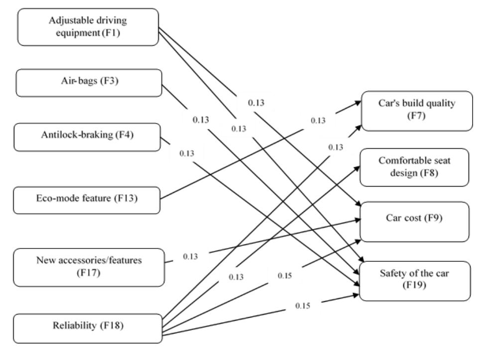
Figure 3 Cause-and-effect relationships.
As we have seen in Figure 3, the sub-factor 'reliability' showed a strong relationship with the sub-factors 'safety of the car' and 'cost of the car', each having a relational strength of 0.15. Other key relationships were obtained between the sub-factors 'reliability' and 'car's build quality' (0.13), as well as between 'reliability' and 'comfortable seat design' (0.13)'.
The result of the above analysis provides valuable insight to designers and higher management people. From Figure 3, it can be understood that key concerns of consumers, such as 'Car cost' and 'Safety of the car', can be managed by the designers by focusing on cause factors such as 'Adjustable driving equipment', 'Air bags' and 'Antilock-braking'. If these features are considered properly in the design of a car, then such a car will have cognitive appeal for consumers and influence their purchasing behavior.
6 Conclusion
Cars are an integral part of many people's lives, whose number is expected to keep increasing in the future. Also, the psychology and purchasing behavior of consumers of cars has been changing over the years. Thus, it is important for car manufacturing companies to understand the psychology of consumers when they buy a car. In this research, various non-visual factors of cars that affect the cognitive behavior of consumers were studied. The non-visual factors were identified through a literature search as well as through a survey of consumers who owned a car or were planning to buy one. Then, the identified factors were analyzed by using the DEMATEL technique to obtain the key factors that affect the cognitive behavior of consumers.
The outcomes of this research indicate that 'Car cost' is the main factor that affects the psychology of car buyers. Consumers perceive that a car with higher cost will grab the attention of people very easily. 'Car cost' is also a key factor in deciding the purchasing capability of consumers. The 'brand value' of a car is another crucial factor that affects the cognitive appeal of consumers. This happens because once a consumer receives information regarding the product through his senses, it remains in their memory, which further drives the purchasing decision. The 'reliability' of the car is another key factor that must be emphasized by car companies to grab the attention of consumers. A car that is perceived as reliable becomes an unbiased choice of consumers in the long term. Some of the factors, such as 'Engine performance' and 'Eco-mode feature', are also important because of their ability to influence most of the other non-visual factors of a car. A car with good engine performance will not only bring a feeling of reliability but also justifies the cost of the car. Thus, the factors mentioned above must be emphasized by the designers while conceptualizing a car. This will help car companies grab the attention of consumers, which will ultimately lead to better sales and increased market share.
The research conducted in this study can be further extended by involving more consumers for a more comprehensive understanding of the non-visual factors of cars that affect the cognitive behavior of consumers. Also, the cognitive behavior of consumers can be better understood by utilizing cognition-based experiments such as eye tracking experiments.
Acknowledgements
Authors acknowledge the Department of Science and Technology, Government of India for financial support vide reference number SR/CSRI/169/2015 (G), under Cognitive Science Research Initiative (CSRI) to carry out this work. We also acknowledge all the respondents and industrial designers who participated.